
Why the correlation gives the best slope#
In which we return to the simple regression problem, and work through the mathematics to show why the correlation is the best least-squares slope for two z-scored arrays.
As background, you may also want to read the regression notation page.
The example regression problem#
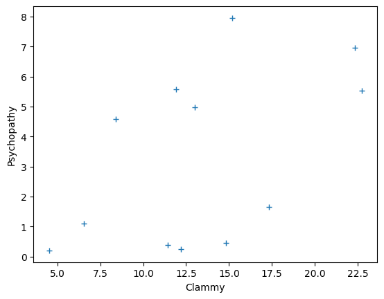
As you remember, we have (fake) measured scores for a “psychopathy” personality trait in 12 students. We also have a measure of how much sweat each student had on their palms, and we call this a “clammy” score.
# Import numerical and plotting libraries
import numpy as np
import numpy.linalg as npl
import matplotlib.pyplot as plt
# Only show 6 decimals when printing
np.set_printoptions(precision=6)
psychopathy = np.array([11.416, 4.514, 12.204, 14.835,
                        8.416,  6.563, 17.343, 13.02,
                        15.19, 11.902, 22.721, 22.324])
clammy = np.array([0.389,  0.2,    0.241,  0.463,
                   4.585,  1.097,  1.642,  4.972,
                   7.957,  5.585,  5.527,  6.964])
plt.plot(psychopathy, clammy, '+')
plt.xlabel('Clammy')
plt.ylabel('Psychopathy');
To get ourselves into a mathematical mood, we will rename our x-axis values to
x and the y-axis values to y. We will store the number of observations in
both as n.
x = psychopathy
y = clammy
n = len(x)
n
12
x and y are Numpy arrays, but we can also call them vectors. Vector is
just a technical and mathematical term for a one-dimensional array.
We are on a quest to find why it turned out that the correlation coefficient is
always the best (least squared error) slope for the z-scored versions of these
vectors (1D arrays). To find out why, we need to express these x and y
vectors in the most general way possible — independent of the numbers we have
here.
\(\newcommand{\yvec}{\vec{y}} \newcommand{\xvec}{\vec{x}} \newcommand{\evec}{\vec{\varepsilon}}\)
First, in mathematical notation, we will call our x array \(\xvec\), to remind
us that x is a vector of numbers, not just a single number.
Next we generalize \(\xvec\) to refer to any set of \(n\) numbers. So, in our x
we have n specific numbers, but we generalize \(\xvec\) to mean a series of \(n\)
numbers, where \(n\) can be any number. We can therefore write \(\xvec\)
mathematically as:
By this we mean that we take \(\xvec\) to be a vector (1D array) of any \(n\) numbers.
By the same logic, we generalize the array y as the vector \(\yvec\):
Writing sums#
We are next going to do the z-score transform on \(\xvec\) and \(\yvec\). As you remember, this involves subtracting the mean and dividing by the standard deviation. We need to express these mathematically.
We will use sum
notation for this
task. This uses the symbol \(\Sigma\) to mean adding up the values in a vector.
\(\Sigma\) is capital S in the Greek alphabet. It is just a shorthand for the
operation we are used to calling sum in code. So:
The \(i\) above is the index for the vector, so \(x_i\) means the element from the vector at position \(i\). So, if \(i = 3\) then \(x_i\) is \(x_3\) — the element at the third position in the vector.
Therefore, in code we, can write \(\Sigma_{i=1}^{n} x_i\) as:
np.sum(x)
160.448
The \(i=1\) and \(n\) at the bottom and top of the \(\Sigma\) mean that adding should start at position 1 (\(x_1\)) and go up to position \(n\) (\(x_n\)). Of course, this means all the numbers in the vector. In this page, we will always sum across all the numbers in the vector, and we will miss off the \(i=1\) and \(n\) above and below the \(\Sigma\), so we will write:
when we mean:
Mean and standard deviation#
Now we have a notation for adding things up in a vector, we can write the mathematical notation for the mean and standard deviation.
We write the mean of a vector \(\xvec\) as \(\xbar\). Say \(\xbar\) as “x bar”. The definition of the mean is:
Read this as add up all the elements in \(\xvec\) and divide by \(n\). In code:
# Calculation of the mean.
x_bar = np.sum(x) / n
x_bar
13.370666666666667
The mean of \(\yvec\) is:
y_bar = np.sum(y) / n
y_bar
3.301833333333333
Next we are going to calculate the standard deviation. In order to do that, we start with the deviations. The deviation for each element is the result of subtracting the mean from the element.
deviations = x - x_bar
deviations
array([-1.954667, -8.856667, -1.166667,  1.464333, -4.954667, -6.807667,
        3.972333, -0.350667,  1.819333, -1.468667,  9.350333,  8.953333])
In mathematical notation, we can write the deviations as:
We have the deviations but we want something called the standard deviation, a measure of how far the typical (standard) value deviates from the mean.
To start, we turn all the deviations to positive values by squaring them. These are the squared deviations:
squared_deviations = deviations ** 2
squared_deviations
array([ 3.820722, 78.440544,  1.361111,  2.144272, 24.548722, 46.344325,
       15.779432,  0.122967,  3.309974,  2.156982, 87.428733, 80.162178])
We can now get an average squared deviation. We can call this the mean squared deviation, but we often call this value — the variance.
# Variance is the mean squared deviation.
variance = np.sum(squared_deviations) / n
variance
28.80166355555556
The standard deviation is the square root of the mean squared deviation — the square root of the variance. We often write the standard deviation as \(\sigma\). Read this as “sigma”. \(\sigma\) is a small “s” in the Greek alphabet.
# Standard deviation
sigma = np.sqrt(variance)
sigma
5.366718136399149
These are simple calculations, but Numpy also has a short-cut to do them, called np.std (NumPy STandard Deviation):
# Numpy calculation of the standard deviation.
np.std(x)
5.366718136399149
We often find ourselves writing equations with the standard deviation \(\sigma\) and the variance (mean squared deviation). Because the variance is the squared standard deviation, we usually write the variance as \(\sigma^2\):
And:
We can be more specific about which vector we are referring to, by adding the vector name as a subscript. For example, if we mean the standard deviation for \(\xvec\), we could write this as \(\sigma_x\):
sigma_x = np.std(x)
sigma_x
5.366718136399149
Similarly for \(\yvec\):
sigma_y = np.std(y)
sigma_y
2.78136974149229
The z-score transformation#
The z-score transformation is to subtract the mean and divide by the standard deviation. Put another way, the z-scores are the deviations divided by the standard deviation:
z_x = (x - x_bar) / sigma_x
z_x
array([-0.36422 , -1.650295, -0.217389,  0.272855, -0.923221, -1.268497,
        0.740179, -0.065341,  0.339003, -0.273662,  1.742281,  1.668307])
z_y = (y - y_bar) / sigma_y
z_y
array([-1.047266, -1.115218, -1.100477, -1.02066 ,  0.461343, -0.792715,
       -0.596768,  0.600484,  1.673696,  0.820879,  0.800025,  1.316677])
Write the z-scores corresponding to \(\xvec\) as \(\zxvec\):
That is the same as saying:
Correlation#
You may remember that the correlation calculation is:
r = np.sum(z_x * z_y) / n
r
0.5178777312914015
In mathematical notation:
Sum of squared error for z-scored lines#
We remind ourselves of the sum of squared error (SSE) for a given slope b and
intercept c.
Here is a function to calculate the sum of squared error for a given x and y vector, slope and intercept:
def calc_sse(x_vals, y_vals, b, c):
    """ Sum of squared error for slope `b`, intercept `c`
    """
    predicted = x_vals * b + c
    errors = y_vals - predicted
    return np.sum(errors ** 2)
Let us start by calculating the SSE values for 1000 intercepts between -1 and 1, and slope of 0.6, using the z-scored x and y values.
n_intercepts = 1000
intercepts = np.linspace(-1, 1, n_intercepts)
sse_inters_b0p6 = np.zeros(n_intercepts)
for i in range(n_intercepts):
    sse_inters_b0p6[i] = calc_sse(z_x, z_y, 0.6, intercepts[i])

plt.plot(intercepts, sse_inters_b0p6)
plt.xlabel('intercept')
plt.ylabel('SSE for intercept, b=0.6');
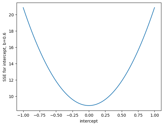
As before, it looks as though \(c=0\) is the intercept that minimizes the SSE, for a slope of 0.6.
Now let us try many slopes, for an intercept of 0.
n_slopes = 1000
slopes = np.linspace(-1, 1, n_slopes)
sse_slopes_c0 = np.zeros(n_slopes)
for i in range(n_slopes):
    sse_slopes_c0[i] = calc_sse(z_x, z_y, slopes[i], 0)

plt.plot(slopes, sse_slopes_c0)
plt.xlabel('slope')
plt.ylabel('SSE for slope, c=0');
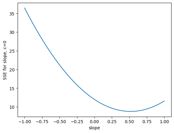
This suggests that the slope minimizing the SSE is around 0.52, at least, for an intercept of 0. It turns out that the correlation value \(r\) above is always the best SSE slope for the z-score line. Our remaining task is to prove this with the mathematical notation we have built up.
Some interesting characteristics of z-scores#
Z-score vectors have a couple of interesting and important mathematical properties.
They have a sum of zero (within the calculation precision of the computer):
np.sum(z_x)
6.661338147750939e-16
Therefore they also have a mean of (near as dammit) zero.
np.mean(z_x)
5.551115123125783e-17
The z-scores have a standard deviation of (near-as-dammit) 1, and therefore, a variance of 1:
np.std(z_x)
0.9999999999999999
This is true for any vector \(\xvec\) (or \(\yvec\)). Why?
To answer that question, we need the results from the algebra of sums. If you read that short page, you fill find that these general results hold:
Addition inside sum#
Multiplication by constant inside sum#
where \(c\) is some constant (number).
Sum of constant value#
Characteristics of z-scores#
With the results above, we can prove z-scores have a sum of 0:
Therefore, it is always true that the sum and mean of a z-score vector are 0.
Next we show z-scores have a variance, and therefore, standard deviation, of 1.
Thus we have learned that:
Because \(\sigma^2_{z_x} = \frac{1}{n} \Sigma (z_{x_i})^2 = 1\):
The least-squares line for z-scores#
Let us say we have a data vector \(\yvec\). We have somehow calculated an estimated (fitted) value \(\hat{y}_i\) for every corresponding value \(y_i\) in \(\yvec\). Then the errors at each value \(i\) are given by:
The sum of squared errors are:
Remembering that \((a + b)^2 = (a + b)(a + b) = a^2 + 2ab + b^2\) we get:
Simplifying with rules of sums above:
Now we introduce our fitted value \(\hat{y}_i\), which we get from our straight line with slope \(b\) and intercept \(c\):
Substituting, then simplifying:
Now, let us assume our \(y_i\) and \(x_i\) values are z-scores. To indicate this, we will use \(z_{y_i}\) and \(z_{x_i}\) instead of \(y_i\) and \(x_i\). As you remember from the results above:
In that case, the equation above simplifies to:
Reality check#
Let us pause at this point for a reality check. If we have done our derivation
correctly, then the formula above should give the same answer as the calc_sse
function above. Let’s check.
def calc_sse_simplified(z_x, z_y, b, c):
    """ Implement simplified z-score SSE equation above
    """
    n = len(z_x)
    return (n - 2 * b * np.sum(z_x * z_y) +
            b ** 2 * n + n * c ** 2)
Does this give the same values as we saw before, for our example intercepts and slope of 0.6?
sse_simplified_b0p6 = np.zeros(n_intercepts)
for i in range(n_intercepts):
    sse_simplified_b0p6[i] = calc_sse_simplified(z_x, z_y, 0.6, intercepts[i])
# Does it give the same results as we got from the original function?
assert np.allclose(sse_simplified_b0p6, sse_inters_b0p6)
How about the example slopes and intercept of 0?
sse_simplified_c0 = np.zeros(n_slopes)
for i in range(n_slopes):
    sse_simplified_c0[i] = calc_sse_simplified(z_x, z_y, slopes[i], 0)
# Does it give the same results as we got from the original function?
assert np.allclose(sse_simplified_c0, sse_slopes_c0)
No errors — we appear to be on the right mathematical track.
Finding the trough in the SSE function#
We want to find the slope, intercept pair \(b, c\) that gives us the lowest SSE value.
To do this, we remind ourselves that the SSE equation above is a function that varies with respect to \(b\) and with respect to \(c\).
Here we plot this function, again, for a variety of values of \(b\):
plt.plot(slopes, sse_simplified_c0)
plt.xlabel('b')
plt.ylabel('SSE for given b, c=0');
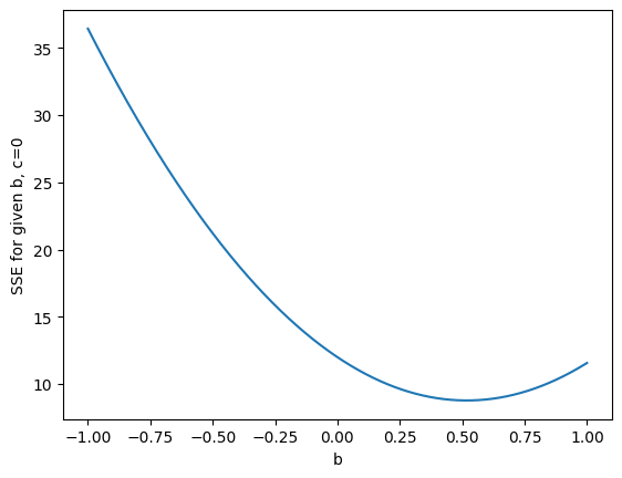
We would like to find the slope \(b\) value corresponding to the minimum of the SSE function. The standard mathematical way to do that is to first make a new function that gives the gradient of the SSE line, at every value for - in our case - \(b\). This new gradient function is called the derivative of the SSE function. Then we find the value of \(b\) for which the gradient (derivative function) is 0. You can see from the graph that the gradient will go to 0 when the function has got to the minimum point, because the gradient is turning from negative to positive. So, when we have found the gradient=0 point, and confirmed it is at the bottom of a trough, as we see in the graph, then we have found the value of \(b\) that minimizes the original SSE function.
We can see the shape of our function curve, and it looks like it is a simple parabola, with one minimum. When we take the derivative of function, which gives us the gradient, we expect to see a single x value where the gradient is 0, and we can see that is a minimum point. But, to be sure about this, in the general case, we will first want to check that there is in fact only one x value for which the derivative is 0. And next, we will want to check whether this point is a minimum point or a maximum point. You can probably imagine that a peak (maximum point) is also going to have a derivative of 0, as the slope goes from positive to negative. In order to check whether a 0 in the derivative is a maximum or a minimum, we take the gradient of the gradient (the derivative of the derivative). This is the second derivative. Think of it as the rate of change of the gradient. If we are at a minimum point, then this rate of change of the gradient is positive, as the gradient goes from negative to positive. If we are at a maximum point, this rate of change of the gradient will be negative, as the gradient goes from positive to negative.
Taking the derivative is also called differentiating the function.
You need to know some rules for taking the derivative, but these rules are not hard to derive, once you are used to the idea of taking the derivative. The key ones rules here are:
You need to know too, that when differentiating with respect to some variable, say \(x\), you can ignore (set to 0) all terms that do not vary with \(x\).
Let us first take the derivative of the \(SSE_z\) function above, with respect to \(c\).
This is zero only when \(c = 0\). Differentiate again to give \(2n\); the second derivative is always positive, so the zero point of the first derivative is a trough (minimum) rather than a peak (maximum).
We have discovered that, regardless of the slope \(b\), the intercept \(c\) that minimizes the sum (and mean) squared error is 0.
Now we have established the always-gives-SSE-minimum value for \(c\), substitute back into the equation above:
Differentiate with respect to \(b\):
This is zero when:
Differentiate again to get:
The second derivative is always positive, so the zero for the first derivative corresponds to a trough (minimum) rather than a peak (maximum).
We have discovered that the slope of the line that minimizes \(SSE_z\) is \(\frac{1}{n} \Sigma z_{x_i} z_{y_i}\) — AKA the correlation.