Slice timing correction

We load and configure libraries to start:

import numpy as np
import matplotlib
import matplotlib.pyplot as plt
plt.rcParams['image.cmap'] = 'gray'  # default gray colormap

import nibabel as nib

import nipraxis

The scanner collected each volume slice by slice. That means that each slice corresponds to a different time.

For example, here is a 4D FMRI image, that we fetch from the web:

# Fetch example image
bold_fname = nipraxis.fetch_file('ds108_sub001_t1r1.nii')
img = nib.load(bold_fname)
data = img.get_fdata()

Downloading file 'ds108_sub001_t1r1.nii' from 'https://raw.githubusercontent.com/nipraxis/nipraxis-data/0.5/ds108_sub001_t1r1.nii' to '/home/runner/.cache/nipraxis/0.5'.

This 4D FMRI image has 24 slices on the third axis (planes, slices in z) and 192 volumes:

data.shape

(64, 64, 24, 192)

The scanner acquired each of these 24 z slices at a different time, relative to the start of the TR.

n_z_slices = data.shape[2]
n_z_slices

24

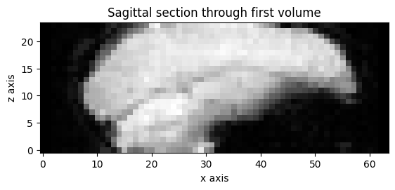
For the moment, let us consider the first volume only.

vol0 = data[..., 0]

Here is a sagittal section showing the z slice positions:

plt.imshow(vol0[31, :, :].T, origin='lower')
plt.title('Sagittal section through first volume')
plt.xlabel('x axis')
plt.ylabel('z axis');

The scanner acquired the slices (planes) in interleaved order, first acquiring slice index 0, 2, 4, … 22 (where 0 is the bottom slice) then acquiring slices 1, 3, 5, .. 23 [1].

Show code cell source Hide code cell source

# Ignore this cell.  It is not relevant to slice timing,
# it just makes the picture.
# Slice indices in space.
space_orders = np.arange(n_z_slices)
# Slice indices in time (acquisition) order.
acq_orders = np.concatenate(
    [space_orders[::2], space_orders[1::2]])
# Acquisition position, ordered by space:
# acq_by_pos[0] is acquisition order of first slice in space,
# acq_by_pos[1] is acquisition order of second slice in space,
# etc.
acq_by_pos = np.argsort(acq_orders)
n_x = n_z_slices * 1.5  # Determines width of picture.
picture = np.repeat(acq_by_pos[:, None], n_x, axis=1)
cm = matplotlib.colors.LinearSegmentedColormap.from_list(
    'light_gray', [[0.4] * 3, [1] * 3])
plt.imshow(picture, cmap=cm, origin='lower')
plt.box(on=False)
plt.xticks([])
plt.yticks(np.arange(n_z_slices))
plt.tick_params(axis='y', which='both', left=False)
plt.ylabel('Position in space (0 = bottom)')
for space_order, acq_order in zip(space_orders, acq_by_pos):
    plt.text(n_x / 2, space_order, str(acq_order), va='center')
plt.title('''\
Slice acquisition order (center) by position (left)

Acquisition order''');

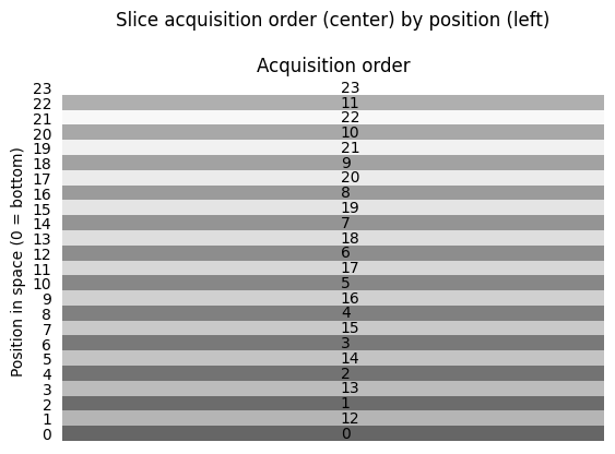
The scanner collected the bottom slice, at slice index 0, at the beginning of the TR, but it collected the next slice in space, at slice index 1, half way through the TR. In this case the time to acquire the whole volume (the TR) was 2.0. The time that the scanner takes to acquire a single slice will be:

TR = 2.0
time_for_single_slice = TR / n_z_slices
time_for_single_slice

0.08333333333333333

The times of acquisition of first and second slices in space (slice 0 and slice 1) will be:

time_for_slice_0 = 0
time_for_slice_1 = time_for_single_slice * n_z_slices / 2
time_for_slice_1

1.0

It may be a problem that different slices correspond to different times.

For example, later on, we may want to run some regression models on these data. We will make a predicted hemodynamic time course and regress the time series (slices over the 4th axis) against this time course. But — it would be convenient if all the voxels in one volume correspond to the same time. Otherwise we would need to sample our hemodynamic prediction at different times for different slices in the z axis.

How can we make a new 4D time series, where all the slices in each volume correspond to our best guess at what these slices would have looked like, if we had acquired them all at the same time?

This is the job of slice timing correction.

Slice timing is interpolation in time

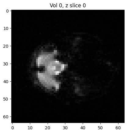
Let’s first get a time series from the bottom slice (in space). Here’s what the bottom slice looks like, for the first volume:

plt.imshow(vol0[:, :, 0])
plt.title('Vol 0, z slice 0');

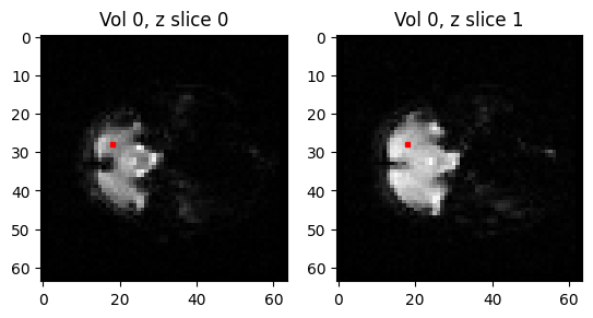
We are going to collect a voxel time series from a sample voxel from this slice, and the slice above it (slice 1):

Our sample voxel coordinates:

vox_x = 28  # voxel coordinate in first dimension
vox_y = 18  # voxel coordinate in second dimension

Here are the coordinates displayed on the images of the slices at position 0 and position 1:

Show code cell source Hide code cell source

fig, axes = plt.subplots(1, 2)
for i in [0, 1]:
    axes[i].imshow(vol0[:, :, i])
    axes[i].set_title(f'Vol 0, z slice {i}')
    # x and y reversed because imshow displays first axis on y.
    axes[i].plot(vox_y, vox_x, 'rs', markersize=3)

We get the time courses from slice 0 and slice 1:

time_course_slice_0 = data[vox_x, vox_y, 0, :]
time_course_slice_1 = data[vox_x, vox_y, 1, :]

The times of acquisition of the voxels for slice 0 are at the beginning of each TR:

vol_nos = np.arange(data.shape[-1])
vol_onset_times = vol_nos * TR
vol_onset_times[:10]

array([ 0.,  2.,  4.,  6.,  8., 10., 12., 14., 16., 18.])

The onset time of the last scan is:

vol_onset_times[-1]

382.0

times_slice_0 = vol_onset_times
times_slice_0[:10]

array([ 0.,  2.,  4.,  6.,  8., 10., 12., 14., 16., 18.])

The times of acquisition of the voxels in slice 1 are half a TR later:

times_slice_1 = vol_onset_times + TR / 2.
times_slice_1[:10]

array([ 1.,  3.,  5.,  7.,  9., 11., 13., 15., 17., 19.])

We can plot the slice 0 time course against slice 0 acquisition time, along with the slice 1 time course against slice 1 acquisition time:

plt.plot(times_slice_0, time_course_slice_0, 'b:+',
    label='slice 0 time course')
plt.plot(times_slice_1, time_course_slice_1, 'r:+',
    label='slice 1 time course')
plt.legend()
plt.title('Time courses for slice 0, slice 1')
plt.xlabel('time (seconds)');

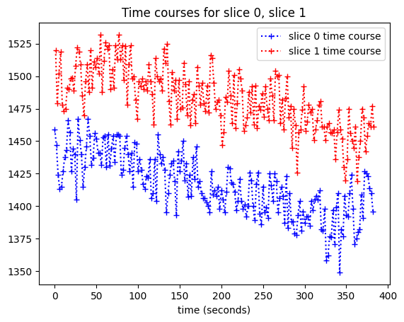
We can’t see the time offset very well here, so let’s plot only the first 10 values (values for the first 10 volumes):

plt.plot(times_slice_0[:10], time_course_slice_0[:10], 'b:+',
    label='slice 0 time course')
plt.plot(times_slice_1[:10], time_course_slice_1[:10], 'r:+',
    label='slice 1 time course')
plt.legend()
plt.title('First 10 values for slice 0, slice 1')
plt.xlabel('time (seconds)');

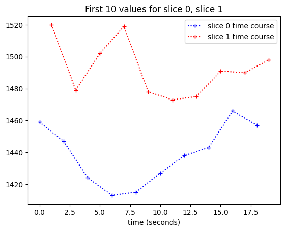
We want to work out a best guess for what the values in slice 1 would be, if we collected them at the beginning of the TR — at the same times as the values for slice 0.

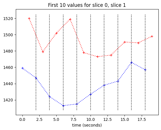
One easy way to do this, might be to do the following for each of our desired samples at times \(t \in 0, 2, 4, ... 382\):

• Draw a vertical line at \(x = t\).

• At the point where the line crosses the slice 1 time course, draw a horizontal line across to the y axis.

• Take this new y value as our interpolation of the slice 1 course, at time \(t\).

Here are the vertical lines at the times of slice 0:

plt.plot(times_slice_0[:10], time_course_slice_0[:10], 'b:+')
plt.plot(times_slice_1[:10], time_course_slice_1[:10], 'r:+')
plt.title('First 10 values for slice 0, slice 1')
plt.xlabel('time (seconds)')
min_y, max_y = plt.ylim()
for i in range(1, 10):
    t = times_slice_0[i]
    plt.plot([t, t], [min_y, max_y], 'k:')

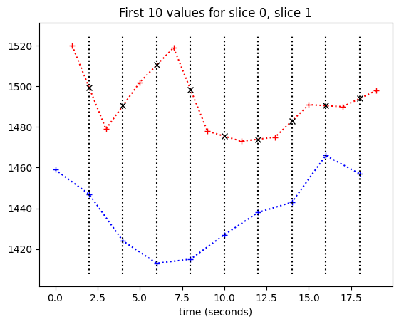
Now we need to work out where these lines cross the slice 1 time course.

This is where we can use Linear interpolation. This is inter-polation because we are estimating a value from the slice 1 time course, that is between two points we do have values for. It is linear interpolation because we are getting our estimate by assuming a straight line between to the two known points in order to estimate our new value.

In the general case of linear interpolation (see Linear interpolation), we have two points, \(x_1, y_1\) and \(x_2, y_2\). In our case we have time on the x axis and voxel values on the y axis.

The formula for the linear interpolation \(y\) value between two points \(x_1, y_1\) and \(x_2, y_2\) is:

\[ y = y_1 + (x-x_1)\frac{y_2-y_1}{x_2-x_1} \]

Now we know the formula for the interpolation, we can apply this to find the interpolated values from the slice 1 time course:

plt.plot(times_slice_0[:10], time_course_slice_0[:10], 'b:+')
plt.plot(times_slice_1[:10], time_course_slice_1[:10], 'r:+')
plt.title('First 10 values for slice 0, slice 1')
plt.xlabel('time (seconds)')
min_y, max_y = plt.ylim()
for i in range(1, 10):
    t = times_slice_0[i]
    plt.plot([t, t], [min_y, max_y], 'k:')
    x = t
    x0 = times_slice_1[i-1]
    x1 = times_slice_1[i]
    y0 = time_course_slice_1[i-1]
    y1 = time_course_slice_1[i]
    # Apply the linear interpolation formula
    y = y0 + (x - x0) * (y1 - y0) / (x1 - x0)
    plt.plot(x, y, 'kx')

It is inconvenient to have to do this calculation for every point. We also need a good way of deciding what to do about values at the beginning and the end.

Luckily Scipy has a sub-package called scipy.interpolate that takes care of this for us.

We use it by first creating an interpolation object, that will do the interpolation. We create this object using the InterpolatedUnivariateSpline class from scipy.interpolate.

from scipy.interpolate import InterpolatedUnivariateSpline as Interp

This class can do more fancy interpolation, but we will use it for linear interpolation (k=1 argument below):

lin_interper = Interp(times_slice_1, time_course_slice_1, k=1)
type(lin_interper)

scipy.interpolate._fitpack2.InterpolatedUnivariateSpline

Our new object knows how to get the linear interpolation between the y values we passed in, given new x values. Here it is in action replicating our manual calculation above.

We use the interpolator to get the values for slice 0 times:

interped_vals = lin_interper(times_slice_0)

plt.plot(times_slice_0[:10], time_course_slice_0[:10], 'b:+')
plt.plot(times_slice_1[:10], time_course_slice_1[:10], 'r:+')
plt.plot(times_slice_0[:10], interped_vals[:10], 'kx')
plt.title('Using the scipy interpolation object');

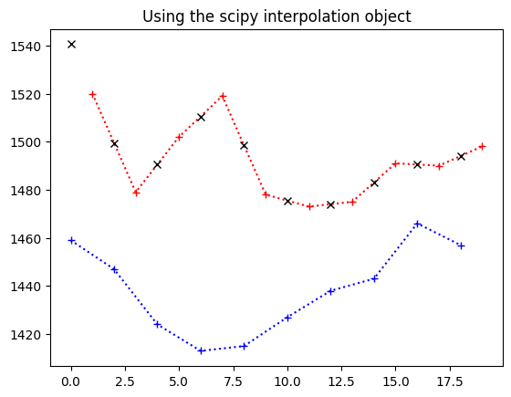
So now we can just replace the original values from the red line (values for slice 1) with our best guess values if the slice had been taken at the same times as slice 0 (black x on the plot). This gives us a whole new time series, that has been interpolated from the original:

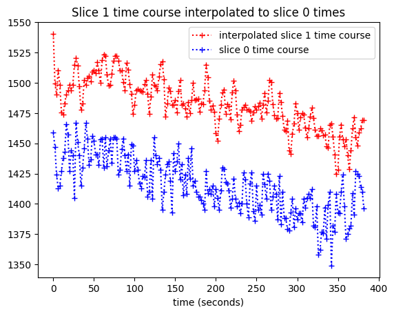
We plot the interpolated time course against the slice 0 times:

plt.plot(times_slice_0, interped_vals, 'r:+',
    label='interpolated slice 1 time course')
plt.plot(times_slice_0, time_course_slice_0, 'b:+',
    label='slice 0 time course')
plt.legend()
plt.title('Slice 1 time course interpolated to slice 0 times')
plt.xlabel('time (seconds)');

Slice time correction

We can do this for each time course in each slice, and make a new 4D image, that has a copy of the values in slice 0, but the interpolated values for all the other slices. This new 4D image has been slice time corrected.

---

[1]

We could not find the slice acquisition order noted in the paper about the relevant study, but the first author, Tor Wager, kindly told us by email. This “ascending-interleaved” order appears to be the default for GE scanners.