Estimation for many voxels at the same time

We often want to fit the same design to many different voxels.

Let’s make a design with a linear trend and a constant term:

import numpy as np
import matplotlib.pyplot as plt
# Print arrays to 2 decimal places
np.set_printoptions(precision=2)

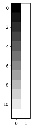
X = np.ones((12, 2))
X[:, 0] = np.linspace(-1, 1, 12)
plt.imshow(X, cmap='gray')

<matplotlib.image.AxesImage at 0x7fd58af1e3e0>

To fit this design to any data, we take the pseudo-inverse:

import numpy.linalg as npl
piX = npl.pinv(X)
piX

array([[-0.21, -0.17, -0.13, -0.1 , -0.06, -0.02,  0.02,  0.06,  0.1 ,
         0.13,  0.17,  0.21],
       [ 0.08,  0.08,  0.08,  0.08,  0.08,  0.08,  0.08,  0.08,  0.08,
         0.08,  0.08,  0.08]])

Notice the shape of the pseudo-inverse:

piX.shape

(2, 12)

Now let’s make some data to fit to. We will draw some samples from the standard normal distribution.

# Random number generator.
rng = np.random.default_rng()
# 12 random numbers from normal distribution, mean 0, std 1.
y_0 = rng.normal(size=12)
y_0

array([ 0.56,  0.95,  0.7 , -0.1 , -0.25, -0.19, -0.76,  0.92,  0.87,
       -0.86, -0.13, -2.05])

beta_0 = piX @ y_0
beta_0

array([-0.8 , -0.03])

We can fit this same design to another set of data, using our already-calculated pseudo-inverse.

y_1 = rng.normal(size=12)
y_1

array([ 0.99,  1.62,  0.31,  1.5 ,  0.21,  0.87,  0.32,  2.4 ,  0.49,
       -0.12,  2.35,  0.5 ])

beta_1 = piX @ y_1
beta_1

array([-0.02,  0.95])

And another!:

y_2 = rng.normal(size=12)
beta_2 = piX @ y_2
beta_2

array([-0.35, -0.38])

Now the trick. Because of the way that matrix multiplication works, we can fit to these three sets of data with the one single matrix multiply:

# Stack the data vectors into columns in a 2D array.
Y = np.stack([y_0, y_1, y_2], axis=1)
Y

array([[ 0.56,  0.99, -1.81],
       [ 0.95,  1.62, -0.02],
       [ 0.7 ,  0.31,  0.08],
       [-0.1 ,  1.5 ,  0.12],
       [-0.25,  0.21, -0.23],
       [-0.19,  0.87, -0.4 ],
       [-0.76,  0.32,  2.18],
       [ 0.92,  2.4 ,  1.18],
       [ 0.87,  0.49, -1.51],
       [-0.86, -0.12, -1.06],
       [-0.13,  2.35, -2.24],
       [-2.05,  0.5 , -0.82]])

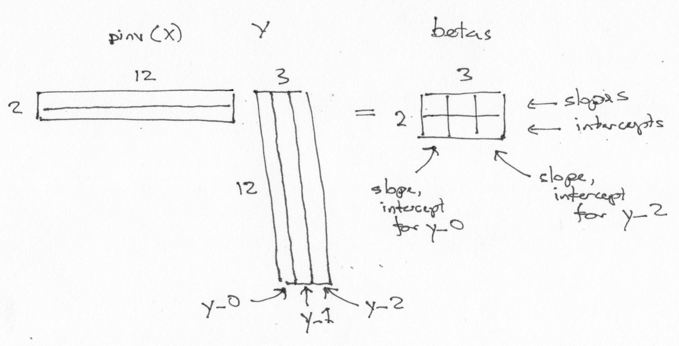
betas = piX @ Y
betas

array([[-0.8 , -0.02, -0.35],
       [-0.03,  0.95, -0.38]])

Notice some features of the betas array:

• There is one row per column in the design X.

• There is one column per column in the data Y.

• The first row of betas contains the parameters corresponding to the first column of the design. The first row therefore contains the slope parameters.

• The second row contains the parameters corresponding to the second column of the design. The second row therefore contains the intercept parameters.

• The first column of betas contains the slope, intercept for the first data vector y_0.

Of course this trick will work for any number of columns of Y.

This trick is important because it allows us to estimate the same design on huge number of data vectors very efficiently. In imaging, this is useful because we can arrange our image data in a one row per volume, one column per voxel array, and use technique here for very fast estimation.