Notation for regression models

Notation for regression models#

# Import numerical and plotting libraries
import numpy as np
import numpy.linalg as npl
import matplotlib.pyplot as plt
# Only show 6 decimals when printing
np.set_printoptions(precision=6)
import scipy.stats as sps

This page starts with the model for simple regression, that you have already see in the regression page.

Our purpose is to introduce the mathematical notation for regression models. You will need this notation to understand the General Linear Model (GLM), a standard statistical generalization of multiple regression. The GLM is the standard model for statistical analysis of functional imaging data.

Sweaty palms, dangerous students#

You have already seen the data we are using here, in the regression page.

We have measured scores for a “psychopathy” personality trait in 12 students. We also measured how much sweat each student had on their palms, and we call this a “clammy” score. We are looking for a straight-line (linear) relationship that allows us to use the “clammy” score to predict the “psychopathy” score.

Here are our particular “psychopathy” and “clammy” scores as arrays:

# The values we are trying to predict.
psychopathy = np.array(
    [11.416,   4.514,  12.204,  14.835,
      8.416,   6.563,  17.343,  13.02,
     15.19 ,  11.902,  22.721,  22.324])

# The values we will predict with.
clammy = np.array(
    [0.389,  0.2  ,  0.241,  0.463,
     4.585,  1.097,  1.642,  4.972,
     7.957,  5.585,  5.527,  6.964])

# The number of values
n = len(clammy)

Here is a plot of the two variables, with clammy on the x-axis and psychopathy on the y-axis. We could refer to this plot as “psychopathy” as a function of “clammy”, where “clammy” is on the x-axis. By convention we put the predictor on the x-axis.

plt.plot(clammy, psychopathy, '+')
plt.xlabel('Clamminess of handshake')
plt.ylabel('Psychopathy score')

Text(0, 0.5, 'Psychopathy score')

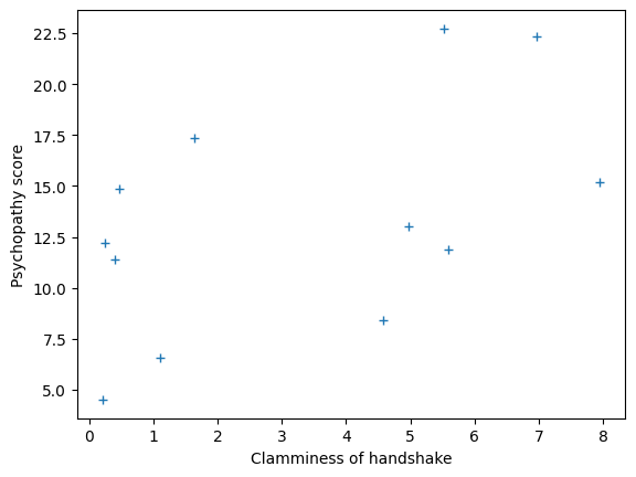
_images/0d0fc12b3cf6e20c9b01a9c76a5ed320fdc809373a23c1f8268d404336f0538b.png

We will call the sequence of 12 “clammy” scores — the “clammy” variable or vector. A vector is a sequence of values — in this case the sequence of 12 “clammy” scores, one for each student. Similarly, we have a “psychopathy” vector of 12 values.

x, y, slope and intercept#

$\newcommand{\yvec}{\vec{y}} \newcommand{\xvec}{\vec{x}} \newcommand{\evec}{\vec{\varepsilon}}$

We could call the “clammy” vector a predictor, but other names for a predicting vector are regressor, covariate, explanatory variable, independent variable or exogenous variable. We also often use the mathematical notation $\xvec$ to refer to a predicting vector. The arrow over the top of $\xvec$ reminds us that $\xvec$ refers to a vector (array, sequence) of values, rather than a single value.

Just to remind us, let’s give the name x to the array (vector) of predicting values:

x = clammy

We could call the vector we are trying to predict the predicted variable, response variable, regressand, dependent variable or endogenous variable. We also often use the mathematical notation $\yvec$ to refer to a predicted vector.

y = psychopathy

You have already seen the best (minimal mean square error) line that relates the clammy (x) scores to the psychopathy (y) scores.

res = sps.linregress(x, y)
res

LinregressResult(slope=0.9992572262138825, intercept=10.071285848579462, rvalue=0.5178777312914014, pvalue=0.0845895203804765, stderr=0.5219718130218388, intercept_stderr=2.2534509778472835)

Call the slope of the line b and the intercept c (C for Constant).

b = res.slope
c = res.intercept

Fitted values and errors#

Remember, our predicted or fitted values are given by multiplying the x (clammy) values by b (the slope) and then adding c (the intercept). In Numpy that looks like this:

fitted = b * x + c
fitted

array([10.459997, 10.271137, 10.312107, 10.533942, 14.65288 , 11.167471,
       11.712066, 15.039593, 18.022376, 15.652137, 15.594181, 17.030113])

The errors are the differences between the fitted and actual (y) values:

errors = y - fitted
errors

array([ 0.956003, -5.757137,  1.891893,  4.301058, -6.23688 , -4.604471,
        5.630934, -2.019593, -2.832376, -3.750137,  7.126819,  5.293887])

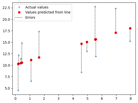
The dashed lines in the plot below represent the errors. The errors values above represent the (positive and negative) lengths of these dashed lines.

# Plot the data
plt.plot(x, y, '+', label='Actual values')
# Plot the predicted values
plt.plot(x, fitted, 'ro', label='Values predicted from line')
# Plot the distance between predicted and actual, for all points.
for i in range(n):
    plt.plot([x[i], x[i]], [fitted[i], y[i]], 'k:')
# The following code line is just to trick Matplotlib into making a new
# a single legend entry for the dotted lines.
plt.plot([], [], 'k:', label='Errors')
# Show the legend
plt.legend()

<matplotlib.legend.Legend at 0x7f61771cefe0>

_images/b4d568c88b2ab68c6ca30ca5a2b0f080d0a48560fc669225795c142654f70055.png

Mathematical notation#

Our next step is to write out this model more generally and more formally in mathematical symbols, so we can think about any vector (sequence) of x values $\xvec$, and any sequence (vector) of matching y values $\yvec$. But to start with, let’s think about the actual set of values we have for $\xvec$. We could write the actual values in mathematical notation as:

\[\begin{split}\displaystyle \vec{x} = [0.389, 0.2, 0.241, 0.463, 4.585, 1.097, \\ \hspace{1.5em}1.642, 4.972, 7.957, 5.585, 5.527, 6.964]\end{split}\]

This means that $\xvec$ is a sequence of these specific 12 values. But we could write $\xvec$ in a more general way, to be any 12 values, like this:

\[\begin{split}\displaystyle \vec{x} = [x_{1}, x_{2}, x_{3}, x_{4}, x_{5}, x_{6}, \\ \hspace{1.5em}x_{7}, x_{8}, x_{9}, x_{10}, x_{11}, x_{12}]\end{split}\]

This means that $\xvec$ consists of 12 numbers, $x_1, x_2 ..., x_{12}$, where $x_1$ can be any number, $x_2$ can be any number, and so on.

$x_1$ is the value for the first student, $x_2$ is the value for the second student, etc.

Here’s another way of looking at the relationship of the values in our particular case, and their notation:

	$\vec{x}$ values	$x$ value notation
1-based index
1	0.389	$x_{1}$
2	0.200	$x_{2}$
3	0.241	$x_{3}$
4	0.463	$x_{4}$
5	4.585	$x_{5}$
6	1.097	$x_{6}$
7	1.642	$x_{7}$
8	4.972	$x_{8}$
9	7.957	$x_{9}$
10	5.585	$x_{10}$
11	5.527	$x_{11}$
12	6.964	$x_{12}$

We can make $\xvec$ be even more general, by writing it like this:

\[ \xvec = [x_1, x_2, ..., x_{n} ] \]

This means that $\xvec$ is a sequence of any $n$ numbers, where $n$ can be any whole number, such as 1, 2, 3 … In our specific case, $n = 12$.

Similarly, for our psychopathy ($\yvec$) values, we can write:

\[\begin{split}\displaystyle \vec{y} = [11.416, 4.514, 12.204, 14.835, 8.416, 6.563, \\ \hspace{1.5em}17.343, 13.02, 15.19, 11.902, 22.721, 22.324]\end{split}\]

	$\vec{y}$ values	$y$ value notation
1-based index
1	11.416	$y_{1}$
2	4.514	$y_{2}$
3	12.204	$y_{3}$
4	14.835	$y_{4}$
5	8.416	$y_{5}$
6	6.563	$y_{6}$
7	17.343	$y_{7}$
8	13.020	$y_{8}$
9	15.190	$y_{9}$
10	11.902	$y_{10}$
11	22.721	$y_{11}$
12	22.324	$y_{12}$

More generally we can write $\yvec$ as a vector of any $n$ numbers:

\[ \yvec = [y_1, y_2, ..., y_{n} ] \]

Notation for fitted values#

If we have $n$ values in $\xvec$ and $\yvec$ then we have $n$ fitted values.

Write the fitted value for the first student as $\hat{y}_1$, that for the second as $\hat{y}_2$, and so on:

\[ \vec{\hat{y}} = [ \hat{y}_1, \hat{y}_2, ..., \hat{y}_n ] \]

Read the $\hat{ }$ over the $y$ as “estimated”, so $\hat{y}_1$ is our estimate for $y_1$, given the model.

Our regression model says each fitted value comes about by multiplying the corresponding $x$ value by $b$ (the slope) and then adding $c$ (the intercept).

So, the fitted values are:

\[\begin{split} \hat{y}_1 = b x_1 + c \\ \hat{y}_2 = b x_2 + c \\ ... \\ \hat{y}_n = b x_n + c \end{split}\]

More compactly:

\[ \vec{\hat{y}} = [ b x_1 + c, b x_2 + c, ..., b x_n + c ] \]

We often use $i$ as a general index into the vectors. So, instead of writing:

\[\begin{split} \hat{y}_1 = b x_1 + c \\ \hat{y}_2 = b x_2 + c \\ ... \\ \hat{y}_n = b x_n + c \end{split}\]

we use $i$ to mean any whole number from 1 through $n$, and so:

\[\begin{split} \hat{y}_i = b x_i + c \\ \text{for } i \in [ 1, 2, ... n] \end{split}\]

For the second line above, read $\in$ as “in”, and the whole line as “For $i$ in 1 through $n$”, or as “Where $i$ can take any value from 1 through $n$ inclusive”.

We mean here, that for any whole number $i$ from 1 through $n$, the fitted value $\hat{y}_i$ (e.g. $\hat{y}_3$, where $i=3$) is given by $b$ times the corresponding $x$ value ($x_3$ where $i=3$) plus $c$.

The error vector $\vec{e}$ is:

\[ \vec{e} = [ e_1, e_2, ..., e_n ] \]

For our linear model, the errors are:

\[\begin{split} \vec{e} = [ y_1 - \hat{y}_1, y_2 - \hat{y}_2, ..., y_n - \hat{y}_n ] \\ = [ y_1 - (b x_1 + c), y_2 - (b x_2 + c), ..., y_n - (b x_n + c) ] \\ \end{split}\]

Again, we could write this same idea with the general index $i$ as:

\[ e_i = y_i - (b x_i + c) \]

Approximation and errors#

Our straight line model says that the $y_i$ values are approximately predicted by the fitted values $\hat{y}_i = b x_i + c$.

\[ y_i \approx bx_i + c \]

Read $\approx$ above as approximately equal to.

With the $\approx$, we are accepting that we will not succeed in explaining our psychopathy values exactly. We can rephrase this by saying that each observation is equal to the predicted value (from the formula above) plus the remaining error for each observation:

\[ y_i = bx_i + c + e_i \]

Of course this must be true for our calculated errors because we calculated them with: