
A worked example of the general linear model#
See: introduction to the general linear model.
Here we go through the matrix formulation of the general linear model with the simplest possible example – a t-test for the difference of the sample mean from zero.
Let us say we have the hypothesis that men are more psychopathic than women.
We find 10 male-female couples, and we give them each a psychopathy questionnaire. We score the questionnaires, and then, for each couple, we subtract the woman’s score from the man’s score, to get a difference score.
We have 10 difference scores:
#: Our standard imports
import numpy as np
import numpy.linalg as npl
# Only show 4 decimals when printing arrays
np.set_printoptions(precision=4)
# Plotting
import matplotlib.pyplot as plt
differences = np.array([ 1.5993, -0.13  ,  2.3806,  1.3761, -1.3595,
                         1.0286,  0.8466,  1.6669, -0.8241,  0.4469])
n = len(differences)
print('Mean', np.sum(differences) / n)
print('STD', np.std(differences))
Mean 0.7031400000000001
STD 1.116777294898137
Our hypothesis is that the females in the couple have a lower psychopathy score. We therefore predict that, in the whole population of male-female couples, the difference measure will, on average, be positive (men have higher scores than women).
We teat this hypothesis by testing whether the sample mean is far enough from zero to make it unlikely that the population mean is actually zero.
To rush ahead, the t-value is always a parameter of interest, in our case, the mean difference, divided by an estimate of the expected variation of that parameter. Specifically, in our case, the value we are expecting for the t-statistic is:
expected_t = np.mean(differences) / (np.std(differences, ddof=1) / np.sqrt(n))
expected_t
1.888845707767012
Here we confirm with the Scipy ttest_1samp function:
import scipy.stats as sps
sps.ttest_1samp(differences, popmean=0)
TtestResult(statistic=1.8888457077670118, pvalue=0.0915047965921625, df=9)
The standard error of the mean#
As you have seen above, the t-statistic requires that we divide the mean value by expected standard deviation of the parameter. The expected standard deviation of the mean is the standard error of the mean.
The standard error of a statistic (such as a mean) is the standard deviation of the sampling distribution of the statistic. The sampling distribution is the distribution of the statistic that we expect when taking a very large number of samples of the statistic. For example, the sampling distribution of the mean, is the expected distribution of the sample means generated by taking a very large number of samples.
What is the standard error of the mean?#
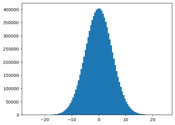
To be more concrete, let’s generate a population with a mean of 0 and a standard deviation of 5.
# The default random number generator in Numpy.
rng = np.random.default_rng()

population = rng.normal(0, 5, size=10000000)

plt.hist(population, bins=100);
As usual, define the mean of a vector of values \(\vec{x}\) as:
# The population mean is near-enough that we'll call it 0
np.sum(population) / len(population)
0.0013791004520730045
# The population standard deviation is near-enough that we'll call it 5
np.std(population)
4.9988543061320865
pop_mean = 0
pop_std = 5
Now imagine we took a sample size n from this population:
n
10
sample = rng.choice(population, size=n, replace=False)
sample
array([  0.7248,  -4.9263,   1.2627,   3.8479,   9.2729, -10.9527,
        -5.5556,   3.7306,  -4.1038,   6.8902])
The sample has a sample mean:
sample_mean = np.mean(sample)   # or np.sum(sample) / n
sample_mean
0.01906234120528936
If I draw a new sample, it will have a different meean. The mean of the sample is itself, somewhat random:
sample = rng.choice(population, size=n, replace=False)
np.mean(sample)
1.4326894762771105
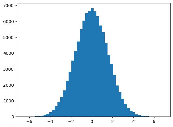
Let us do that many times, to get an idea of the distribution of the means from samples of size n. This is called the sampling distribution of the mean:
n_samples = 100000
sample_means = np.zeros(n_samples)
for i in range(n_samples):
    sample = rng.choice(population, size=n, replace=False)
    sample_means[i] = np.mean(sample)
sample_means[:10]
array([ 0.2273,  1.8352, -2.0397,  0.7912, -2.8466,  0.4882, -2.4278,
       -1.4564,  1.4205,  0.6521])
We now have the sampling distribution of the mean:
plt.hist(sample_means, bins=50);
The standard error of the mean is nothing but the estimate, using some assumptions of the standard deviation of this distribution. For example, for our particular n_samples samples, we got a sampling distribution standard deviation of:
# Standard deviation of sampling distribution of mean.
np.std(sample_means)
1.5778529309128413
The standard error of the mean (SEM) is an estimate of this value using some assumptions, but without having to draw multiple samples from the population. It is given by the population standard deviation divided by the square root of n:
pop_sem = pop_std / np.sqrt(n)
pop_sem
1.5811388300841895
Notice that the SEM is very close to our estimate by drawing lots of samples. Our estimate will, of course, be a little random, because it depends on the exact random samples we drew from the population.
But wait!, I hear you cry, we usually don’t know the standard deviation of the population. Often, even usually, all we have to go on is the sample. We need an estimate of the standard deviation, to give an estimate for the standard error of the mean.
One estimate could be the standard deviation of the sample we have, as in:
np.std(sample)
4.434331394678495
As you may remember, the Numpy calculation for the standard deviation is:
In code, this is:
# Numpy calculation
variance = np.sum((sample - np.mean(sample)) ** 2) / n
sigma = np.sqrt(variance)
sigma
4.434331394678495
Unfortunately, this is not the best number to use, because it turns out this calculation of the standard deviation tends to be lower than the population standard deviation, for reasons related to the fact that we used the sample mean to calculate the standard deviation. In technical terms, this calculation is biased to be too low, on average, compared to the population standard deviation.
We have to do a small correction for this effect, by dividing the variance by \(n - 1\) rather than \(n\). This version of the calculation produces an unbiased estimate of population standard deviation:
So, the unbiased estimate of the standard deviation of \(\vec{x}\) as:
In code:
v_u = np.sum((sample - np.mean(sample)) ** 2) / (n - 1)
s_u = np.sqrt(v_u)
s_u
4.674195702391699
Numpy does this calculation if we pass ddof=1 to the std function. ddof stands for Delta Degrees of Freedom, and refers to the number of parameters we had to estimate to calculate the standard deviation. In our current case, this is 1, for the mean.
np.std(sample, ddof=1)
4.674195702391699
The unbiased Standard Error of the Mean (SEM) from the sample uses the unbiased standard deviation from the sample, and is:
where \(n\) is the number of samples, in our case:
n
10
Therefore:
SEM_u = s_u / np.sqrt(n)
SEM_u
1.4781104648928314
Notice that this isn’t far from the SEM calculated from the population standard deviation, or from the standard deviation of the sampling distribution that we calculated by taking many samples, but this estimate of the SEM will vary from sample to sample, as the mean and unbiased standard deviation will vary.
t statistic, SEM#
A t statistic is given by a value divided by the standard error of that value. The t statistic for \(\bar{x}\) is:
In our case:
x = differences
n = len(x)
x_bar = np.mean(x)
x_bar
0.7031400000000001
unbiased_var_x = 1. / (n - 1) * np.sum((x - x_bar) ** 2)
s_x = np.sqrt(unbiased_var_x)
s_x
1.1771866303465508
# Unbiased SEM uses the unbiased standard deviation
SEM = s_x / np.sqrt(n)
SEM
0.3722590982993789
t = x_bar / SEM
t
1.888845707767012
Testing using the general linear model#
It is overkill for us to use the general linear model for this, but it does show how the machinery works in the simplest case.
\(\newcommand{Xmat}{\boldsymbol X} \newcommand{\bvec}{\vec{\beta}}\) \(\newcommand{\yvec}{\vec{y}} \newcommand{\xvec}{\vec{x}} \newcommand{\evec}{\vec{\varepsilon}}\)
The matrix expression of the general linear model is:
\(\newcommand{Xmat}{\boldsymbol X} \newcommand{\bvec}{\vec{\beta}}\)
Define our design matrix \(\Xmat\) to have a single column of ones:
X = np.ones((n, 1))
X
array([[1.],
       [1.],
       [1.],
       [1.],
       [1.],
       [1.],
       [1.],
       [1.],
       [1.],
       [1.]])
\(\newcommand{\bhat}{\hat{\bvec}} \newcommand{\yhat}{\hat{\yvec}}\)
\(\bhat\) is The least squares estimate for \(\bvec\), and is given by:
Because \(\Xmat\) is just a column of ones, \(\Xmat^T \yvec = \sum_i{y_i}\).
\(\Xmat^T \Xmat = n\), so \((\Xmat^T \Xmat)^{-1} = \frac{1}{n}\).
Thus:
pX = npl.pinv(X)
pX
array([[0.1, 0.1, 0.1, 0.1, 0.1, 0.1, 0.1, 0.1, 0.1, 0.1]])
B = pX @ differences
assert np.isclose(B, np.mean(differences))
The student’s t statistic from the general linear model is:
where \(\hat{\sigma}^2\) is our estimate of variance in the residuals, \(c\) is a contrast vector to select some combination of the design columns, and \((\Xmat^T \Xmat)^+\) is the pseudoinverse of \(\Xmat^T \Xmat\).
In our case we have only one design column, so \(c = [1]\) and we can omit it. \(\hat{\sigma}^2 = s_x^2\) for \(s_x\) defined above. \(\Xmat^T \Xmat\) is invertible, and we know the inverse already: \(\frac{1}{n}\).
iXtX = npl.inv(X.T @ X)
assert np.isclose(iXtX, 1 / n)
Therefore:
s_x = np.sqrt(np.sum((differences - np.mean(differences)) ** 2) / (n - 1))
t = B / (s_x * np.sqrt(iXtX))
t
array([[1.8888]])