Regression for a single voxel

Earlier – Voxel time courses – we were looking at a single voxel time course.

Here we use simple regression to do a test on a single voxel.

Let’s get that same voxel time course back again:

import numpy as np
import matplotlib.pyplot as plt
import nibabel as nib
# Only show 6 decimals when printing
np.set_printoptions(precision=6)

We load the data, and knock off the first four volumes to remove the artefact we discovered in First go at brain activation exercise:

# Load the function to fetch the data file we need.
import nipraxis
# Fetch the data file.
data_fname = nipraxis.fetch_file('ds114_sub009_t2r1.nii')
# Show the file name of the fetched data.
data_fname

'/home/runner/.cache/nipraxis/0.5/ds114_sub009_t2r1.nii'

img = nib.load(data_fname)
data = img.get_fdata()
data = data[..., 4:]

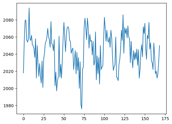
The voxel coordinate (3D coordinate) that we were looking at in Voxel time courses was at (42, 32, 19):

voxel_time_course = data[42, 32, 19]
plt.plot(voxel_time_course)

[<matplotlib.lines.Line2D at 0x7fb10c248760>]

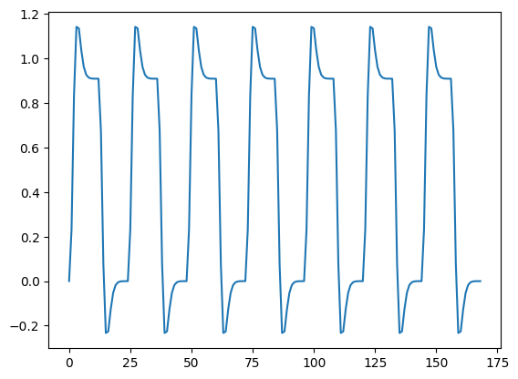
Now we are going to use the convolved regressor from Convolving with the hemodyamic response function to do a simple regression on this voxel time course.

First fetch the text file with the convolved time course:

tc_fname = nipraxis.fetch_file('ds114_sub009_t2r1_conv.txt')
# Show the file name of the fetched data.
tc_fname

'/home/runner/.cache/nipraxis/0.5/ds114_sub009_t2r1_conv.txt'

convolved = np.loadtxt(tc_fname)
# Knock off first 4 elements to match data
convolved = convolved[4:]
plt.plot(convolved)

[<matplotlib.lines.Line2D at 0x7fb10c1348e0>]

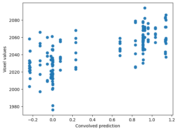
Finally, we plot the convolved prediction and the time-course together:

plt.scatter(convolved, voxel_time_course)
plt.xlabel('Convolved prediction')
plt.ylabel('Voxel values')

Text(0, 0.5, 'Voxel values')

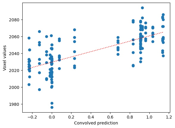
Using correlation-like calculations

We can get the best-fitting line using the calculations from the regression page:

def calc_z_scores(arr):
    """ Calculate z-scores for array `arr`
    """
    return (arr - np.mean(arr)) / np.std(arr)

# Correlation
r = np.mean(calc_z_scores(convolved) * calc_z_scores(voxel_time_course))
r

0.7044637722561977

The best fit line is:

best_slope = r * np.std(voxel_time_course) / np.std(convolved)
print('Best slope:', best_slope)
best_intercept = np.mean(voxel_time_course) - best_slope * np.mean(convolved)
print('Best intercept:', best_intercept)

Best slope: 31.185513664914524
Best intercept: 2029.367689291584

plt.scatter(convolved, voxel_time_course)
x_vals = np.array([np.min(convolved), np.max(convolved)])
plt.plot(x_vals, best_intercept + best_slope * x_vals, 'r:')
plt.xlabel('Convolved prediction')
plt.ylabel('Voxel values')

Text(0, 0.5, 'Voxel values')

Using Scipy:

import scipy.stats as sps
sps.linregress(convolved, voxel_time_course)

LinregressResult(slope=31.18551366491453, intercept=2029.367689291584, rvalue=0.7044637722561978, pvalue=1.1832511547748845e-26, stderr=2.4312815394118448, intercept_stderr=1.634742742490283)