Resampling with scipy.ndimage

# import common modules
import numpy as np
np.set_printoptions(precision=4)  # print arrays to 4DP
import matplotlib.pyplot as plt
plt.rcParams['image.cmap'] = 'gray'

Reampling, pull, push

Let us say we have two images \(\mathbf{I}\) and \(\mathbf{J}\).

There is some spatial transform between them, such as a translation, or rotation.

We could either think of the transformation that maps \(\mathbf{I} \to \mathbf{J}\) or \(\mathbf{J} \to \mathbf{I}\).

The transformations map voxel coordinates in one image to coordinates in the other.

For example, write a coordinate in \(\mathbf{I}\) as \((x_i, y_i, z_i)\), and a coordinate in \(\mathbf{J}\) as \((x_j, y_j, z_j)\).

The mapping \(\mathbf{I} \to \mathbf{J}\) maps \((x_i, y_i, z_i) \to (x_j, y_j, z_j)\).

Now let us say that we want to move image \(\mathbf{J}\) to match image \(\mathbf{I}\).

To do this moving, we need to resample \(\mathbf{J}\) onto the same voxel grid as \(\mathbf{I}\).

Specifically, we are going to do the following:

• make a new empty image \(\mathbf{K}\) that has the same voxel grid as \(\mathbf{I}\);

• for each coordinate in \(\mathbf{I} : (x_i, y_i, z_i)\) we will apply the transform \(\mathbf{I} \to \mathbf{J}\) to get \((x_j, y_j, z_j)\);

• we will probably need to estimate a value \(v\) from \(\mathbf{J}\) at \((x_j, y_j, z_j)\) because the coordinate values \((x_j, y_j, z_j)\) will probably not be integers, and so there is no exactly matching value in \(\mathbf{J}\);

• we place \(v\) into \(\mathbf{K}\) at coordinate \((x_i, y_i, z_i)\).

Notice that, in order to move \(\mathbf{J}\) to match \(\mathbf{I}\) we needed the opposite transform – that is: \(\mathbf{I} \to \mathbf{J}\). This is called pull resampling.

We will call the \(\mathbf{I} \to \mathbf{J}\) transform the resampling transform.

Scipy ndimage and affine_transform

Scipy has a function for doing reampling with transformations, called scipy.ndimage.affine_transform.

from scipy.ndimage import affine_transform

It does all the heavy work of resampling for us.

For example, lets say we have an image volume \(\mathbf{I}\) (ds107_sub012_t1r2.nii):

# Fetch the data file.
import nipraxis
# Fetch image file.
bold_fname = nipraxis.fetch_file('ds107_sub012_t1r2.nii')
bold_fname

'/home/runner/.cache/nipraxis/0.5/ds107_sub012_t1r2.nii'

import nibabel as nib
img = nib.load(bold_fname)
data = img.get_fdata()
I = data[..., 0]  # I is the first volume

We have another image volume \(\mathbf{J}\):

J = data[..., 1]  # I is the second volume

Let’s say we know that the resampling transformation \(\mathbf{I} \to \mathbf{J}\) is given by:

• a rotation by 0.2 radians about the x axis;

• a translation of [1, 2, 3] voxels.

See Rotations and rotation matrices for more on 2D and 3D rotation matrices.

Here we use the nipraxis.rotations module. It has routines that will make 3 by 3 rotation matrices for rotations by given angles around the x, y, and z axes.

Of course you will want to be assured these functions are tested. Have a look at test_rotations.py.

We use the routines in the nipraxis.rotations module to make the rotation matrix we need:

from nipraxis.rotations import x_rotmat
# rotation matrix for rotation of 0.2 radians around x axis
M = x_rotmat(0.2)
M
translation = [1, 2, 3]  # Translation from I to J
translation

[1, 2, 3]

The affine_transform function does the work of resampling. By default, it implements the following algorithm:

• makes the new empty volume K, assuming it will be the same shape as J;

• for each coordinate \((x_i, y_i, z_i)\) implied by the volume K:

  • apply the transformations implied by M and translation to \((x_i, y_i, z_i)\) to get the corresponding point in J : \((x_j, y_j, z_j)\);

  • resample J at \((x_j, y_j, z_j)\) to get \(v\);

  • place \(v\) at \((x_i, y_i, z_i)\) in K

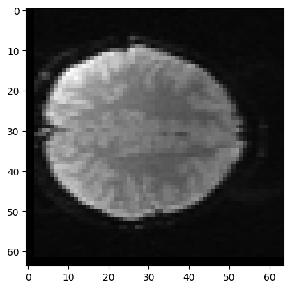
# order=1 for linear interpolation
K = affine_transform(J, M, translation, order=1)
K.shape
plt.imshow(K[:, :, 17])

<matplotlib.image.AxesImage at 0x7f9131da1510>

Resampling with images of different shapes

Notice the assumption that affine_transform makes above – that the output image will be the same shape as the input image.

This need not be the case. In fact we can tell affine_transform to start with an empty volume K with another shape. To do this, we use the output_shape parameter.

Now we can be more precise about the algorithm of affine_transform. affine_transform accepts:

• input – an array to resample from. Say this array as n dimensions (len(input.shape));

• matrix – an n by n transformation matrix (the top left mat part of an affine);

• offset – a optional length n translation vector to be applied after the matrix transformation (the vec part of an affine);

• output_shape : an optional tuple giving the shape of the output array into which we will put the values resampled from input. output_shape defaults to input.shape; this is the default we have been using above.

affine_transform then generates all the voxel coordinates implied by the output_shape, and transforms them with the matrix and offset transforms to get a new set of coordinates C. It then samples the input array at the coordinates given by C to generate the output array.

Here is the call to affine_transform that we used above, where we allowed the routine to assume that the output shape was the same as the input shape:

K = affine_transform(J, M, translation, order=1)
K.shape

(64, 64, 35)

The is the same as the following call, where we specify the shape explicitly:

K = affine_transform(J, M, translation, output_shape=J.shape, order=1)
K.shape

(64, 64, 35)

The output shape can be different from the input shape:

K = affine_transform(J, M, translation,
                     output_shape=(65, 65, 36), order=1)
K.shape

(65, 65, 36)

Remember that the M matrix and translation vector apply to the coordinates implied by the output shape.