
Correlating with voxel time courses#
When we have a 4D image, we can think of the data in several ways. For example the data could be:
A series of 3D volumes (slicing over the last axis);
A collection of 1D voxel time courses (slicing over the first three axes).
# Our usual set-up
import numpy as np
import matplotlib.pyplot as plt
# Display array values to 4 digits of precision
np.set_printoptions(precision=4, suppress=True)
# Load the function to fetch the data file we need.
import nipraxis
# Fetch the data file.
data_fname = nipraxis.fetch_file('ds114_sub009_t2r1.nii')
# Show the file name of the fetched data.
data_fname
'/home/runner/.cache/nipraxis/0.5/ds114_sub009_t2r1.nii'
We load a 4D file:
import nibabel as nib
img = nib.load(data_fname)
img.shape
(64, 64, 30, 173)
We drop the first volume; as you remember, the first volume is very different from the rest of the volumes in the series:
# Drop the first volume
data = img.get_fdata()
data = data[..., 1:]
data.shape
(64, 64, 30, 172)
As you have seen in the 4D introduction, we can think of this 4D data as a series of 3D volumes. That is the way we have been thinking of the 4D data so far:
# This is slicing over the last (time) axis
vol0 = data[..., 0]
vol0.shape
(64, 64, 30)
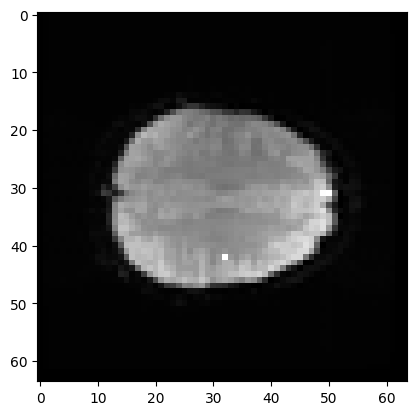
In that page, we found a 3D coordinate for an interesting voxel. The 3D coordinate is just the indices in the first three dimensions — the dimensions representing space. We can write the coordinate as indices in a tuple like
this: (42, 32, 19). As you saw in the 4D page, the first index of 42 refers
to a position towards the left of the brain (> 31). The second index of 32
refers to a position almost in the center front to back. The last index of 19
refers to a position a little further towards the top of the brain – in this
image.
Here is the position of that coordinate displayed on a plane of the 3D volume (in fact, the mean volume).
# Where is this in the brain?
mean_data = np.mean(data, axis=-1)
# Make a nice bright dot in the right place
mean_data[42, 32, 19] = np.max(mean_data)
plt.imshow(mean_data[:, :, 19], cmap='gray')
<matplotlib.image.AxesImage at 0x7fc100287dc0>
If I slice into the data array with these coordinates, I will get a vector, with the image value at that position (43, 32, 19), for every point in time:
# This is slicing over all three of the space axes
voxel_time_course = data[42, 32, 19]
print(voxel_time_course.shape)
plt.plot(voxel_time_course)
(172,)
[<matplotlib.lines.Line2D at 0x7fc1001e2fb0>]
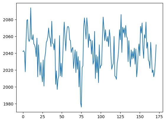
This is a “voxel time course”.
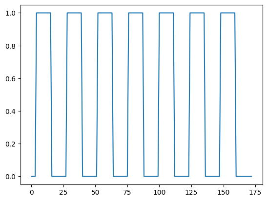
We might want to do ordinary statistical type things with this time course. For example, we might want to correlate this time course with a measure of whether the subject was doing the task or not.
This measure will have 1 for each volume (time point) where the subject was doing the task, and 0 for each volume where the subject was at rest.
We call this a “neural” time course, because we believe that the nerves in the relevant brain area will switch on when the task starts (value = 1) and then switch off when the task stops (value = 0).
To get this on-off measure, we will use our pre-packaged function for OpenFMRI data:
# Fetch the condition file
import nipraxis

cond_fname = nipraxis.fetch_file('ds114_sub009_t2r1_cond.txt')
cond_fname
'/home/runner/.cache/nipraxis/0.5/ds114_sub009_t2r1_cond.txt'
# Load the neural time course using pre-packaged function
from nipraxis.stimuli import events2neural
TR = 2.5  # time between volumes
n_trs = img.shape[-1]  # The original number of TRs
neural = events2neural(cond_fname, TR, n_trs)
plt.plot(neural)
[<matplotlib.lines.Line2D at 0x7fc10005a3b0>]
Here we plot the voxel time course against this neural prediction:
# Plot the neural prediction against the data
neural = neural[1:]
# Notice the 'o' to specify the "line marker"
plt.plot(neural, voxel_time_course, 'o')
# Set the axis limits to give space on left and right
axis = plt.gca()
axis.set_xlim(-0.1, 1.1)
(-0.1, 1.1)
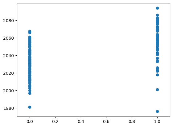
We can look at the correlation between the on-off prediction and the voxel time course:
# Correlate the neural time course with the voxel time course
corr_array = np.corrcoef(neural, voxel_time_course)
corr_array
array([[1.    , 0.5429],
       [0.5429, 1.    ]])
Notice that Numpy has correlated neural with neural — to give 1 — and voxel_time_course, to give:
# Correlation of neural (row 0) with voxel_time_course (column 1)
correlation = corr_array[0, 1]
correlation
0.5428503395516837
In the same way it has correlated voxel_time_course with neural and voxel_time_course, to give a 2 by 2 array.
A reminder on correlation#
We are sure that correlation is familiar to you, but here we define it, as a reminder.
Correlation between two 1D arrays is the result of converting each array to z-scores, element-wise multiplying the z-score arrays, and taking the mean of the result.
Turning an array into a z-score (AKA standard score) is the operation of:
Subtracting the mean of the array then
Dividing by the standard deviation.
Let’s do that for the two arrays above:
# z-scores for voxel_time_course.
vtc_mean = np.mean(voxel_time_course)
vtc_std = np.std(voxel_time_course)
vtc_z_scores = (voxel_time_course - vtc_mean) / vtc_std
# Show the first 10 values.
vtc_z_scores[:10]
array([-0.0652, -0.0194, -0.1109, -1.163 ,  0.4837,  1.6273,  1.673 ,
        0.621 ,  0.4837,  0.621 ])
# z-scores for neural time course
neural_mean = np.mean(neural)
neural_std = np.std(neural)
neural_z_scores = (neural - neural_mean) / neural_std
neural_z_scores[:10]
array([-0.977 , -0.977 , -0.977 ,  1.0235,  1.0235,  1.0235,  1.0235,
        1.0235,  1.0235,  1.0235])
Now we multiply them together, using the usual element by element Numpy multiplication rules for arrays:
multiplied = vtc_z_scores * neural_z_scores
multiplied[:10]
array([ 0.0637,  0.019 ,  0.1083, -1.1903,  0.4951,  1.6656,  1.7124,
        0.6356,  0.4951,  0.6356])
To calculate the correlation, we take the mean:
correlation_again = np.mean(multiplied)
correlation_again
0.5428503395516836
This recalculation is very very close to the original. The difference is so tiny we can put it down to floating point error.
np.isclose(correlation, correlation_again)
True