Convolution

Neural and hemodynamic models

In functional MRI (FMRI), we often have the subjects do a task in the scanner. For example, we might have the subject lying looking at a fixation cross on the screen for most of the time, and sometimes show a very brief burst of visual stimulation, such as a flashing checkerboard.

We will call each burst of stimulation an event.

The FMRI signal comes about first through changes in neuronal firing, and then by blood flow responses to the changes in neuronal firing. In order to predict the FMRI signal to an event, we first need a prediction (model) of the changes in neuronal firing, and second we need a prediction (model) of how the blood flow will change in response to the neuronal firing.

So we have a two-stage problem:

• predict the neuronal firing to the event (make a neuronal firing model);

• predict the blood flow changes caused by the neuronal firing (a hemodynamic model).

Convolution is a simple way to create a hemodynamic model from a neuronal firing model.

The neuronal firing model

The neuronal firing model is our prediction of the profile of neural activity in response to the event.

For example, in this case, with a single stimulation, we might predict that, as soon as the visual stimulation went on, the cells in the visual cortex instantly increased their firing, and kept firing at the same rate while the stimulation was on.

In that case, our neural model of an event starting at 4 seconds, lasting 5 seconds, might look like this:

import numpy as np
import matplotlib.pyplot as plt

times = np.arange(0, 40, 0.1)
n_time_points = len(times)
neural_signal = np.zeros(n_time_points)
neural_signal[(times >= 4) & (times < 9)] = 1
plt.plot(times, neural_signal)
plt.xlabel('time (seconds)')
plt.ylabel('neural signal')
plt.ylim(0, 1.2)
plt.title("Neural model for 5 second event starting at time 4")

Text(0.5, 1.0, 'Neural model for 5 second event starting at time 4')

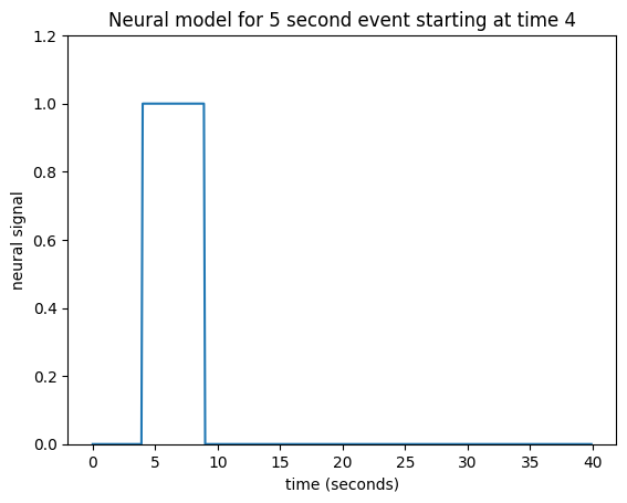
This type of simple off - on - off model is a boxcar function.

Of course we could have had another neural model, with the activity gradually increasing, or starting high and then dropping, but let us stick to this simple model for now.

Now we need to predict our hemodynamic signal, given our prediction of neuronal firing.

The impulse response

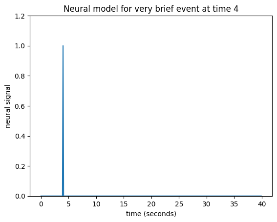
Let’s simplify a little by specifying that the event was really short. Call this event — an impulse. This simplifies our neural model to a single spike in time instead of the sustained rise of the box-car function.

neural_signal = np.zeros(n_time_points)
i_time_4 = np.where(times == 4)[0][0]  # index of value 4 in "times"
neural_signal[i_time_4] = 1  # A single spike at time == 4
plt.plot(times, neural_signal)
plt.xlabel('time (seconds)')
plt.ylabel('neural signal')
plt.ylim(0, 1.2)
plt.title("Neural model for very brief event at time 4")

Text(0.5, 1.0, 'Neural model for very brief event at time 4')

Let us now imagine that I know what the hemodynamic response will be to such an impulse. I might have got this estimate from taking the FMRI signal following very brief events, and averaging over many events. Here is one such estimate of the hemodynamic response to a very brief stimulus:

def hrf(t):
    "A hemodynamic response function"
    return t ** 8.6 * np.exp(-t / 0.547)

hrf_times = np.arange(0, 20, 0.1)
hrf_signal = hrf(hrf_times)
plt.plot(hrf_times, hrf_signal)
plt.xlabel('time (seconds)')
plt.ylabel('BOLD signal')
plt.title('Estimated BOLD signal for event at time 0')

Text(0.5, 1.0, 'Estimated BOLD signal for event at time 0')

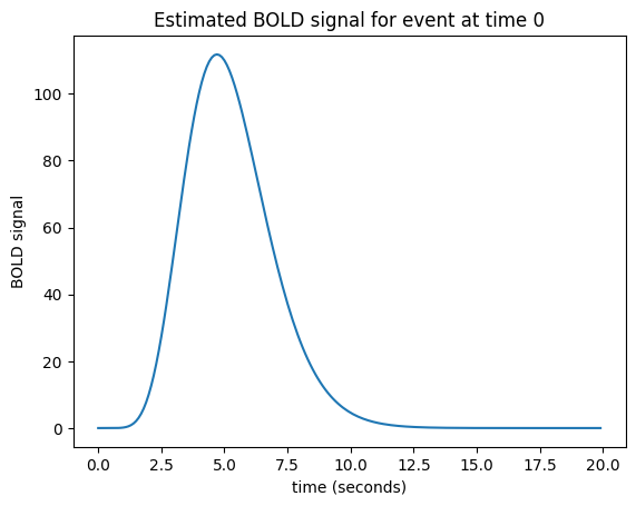
This is the hemodynamic response to a neural impulse. In signal processing terms this is the hemodynamic impulse response function. It is usually called the hemodynamic response function (HRF), because it is a function that gives the predicted hemodynamic response at any given time following an impulse at time 0.

Building the hemodynamic output from the neural input

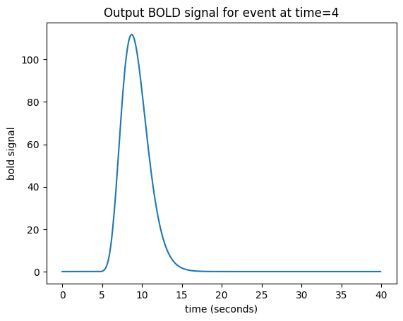
We now have an easy way to predict the hemodynamic output from our single impulse at time 4. We take the HRF (prediction for an impulse starting at time 0), and shift it by 4 seconds-worth to give our predicted output:

n_hrf_points = len(hrf_signal)
bold_signal = np.zeros(n_time_points)
bold_signal[i_time_4:i_time_4 + n_hrf_points] = hrf_signal
plt.plot(times, bold_signal)
plt.xlabel('time (seconds)')
plt.ylabel('bold signal')
plt.title('Output BOLD signal for event at time=4')

Text(0.5, 1.0, 'Output BOLD signal for event at time=4')

Our impulse so far has an amplitude of 1. What if the impulse was twice as strong, with an amplitude of 2?

neural_signal[i_time_4] = 2  # An impulse with amplitude 2
plt.plot(times, neural_signal)
plt.xlabel('time (seconds)')
plt.ylabel('neural signal')
plt.ylim(0, 2.2)
plt.title('Neural model for amplitude 2 impulse')

Text(0.5, 1.0, 'Neural model for amplitude 2 impulse')

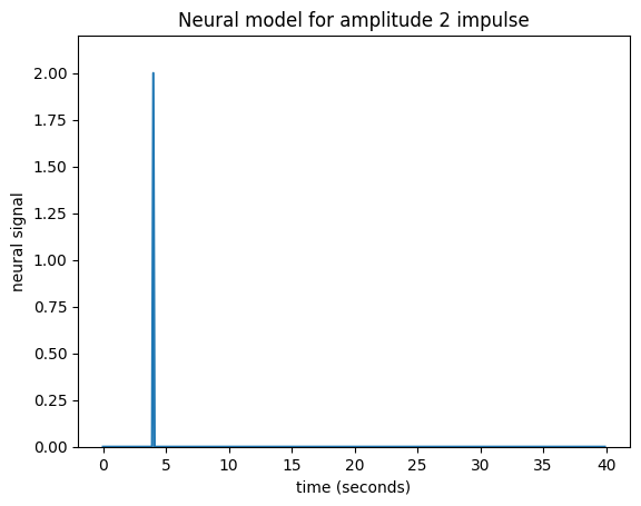
Maybe I can make the assumption that, if the impulse is twice as large then the response will be twice as large. This is the assumption that the response scales linearly with the impulse.

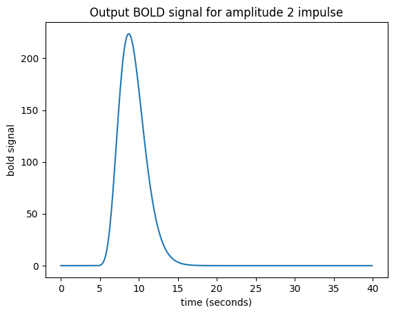
Now I can predict the output for an impulse of amplitude 2 by taking my HRF, shifting by 4, as before, and then multiplying the HRF by 2:

bold_signal = np.zeros(n_time_points)
bold_signal[i_time_4:i_time_4 + n_hrf_points] = hrf_signal * 2
plt.plot(times, bold_signal)
plt.xlabel('time (seconds)')
plt.ylabel('bold signal')
plt.title('Output BOLD signal for amplitude 2 impulse')

Text(0.5, 1.0, 'Output BOLD signal for amplitude 2 impulse')

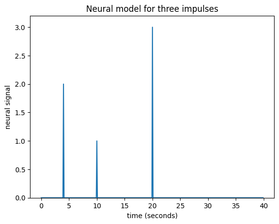
What if I have several impulses? For example, imagine I had an impulse amplitude 2 at time == 4, then another of amplitude 1 at time == 10, and another of amplitude 3 at time == 20.

neural_signal[i_time_4] = 2  # An impulse with amplitude 2
i_time_10 = np.where(times == 10)[0][0]  # index of value 10 in "times"
neural_signal[i_time_10] = 1  # An impulse with amplitude 1
i_time_20 = np.where(times == 20)[0][0]  # index of value 20 in "times"
neural_signal[i_time_20] = 3  # An impulse with amplitude 3
plt.plot(times, neural_signal)
plt.xlabel('time (seconds)')
plt.ylabel('neural signal')
plt.ylim(0, 3.2)
plt.title('Neural model for three impulses')

Text(0.5, 1.0, 'Neural model for three impulses')

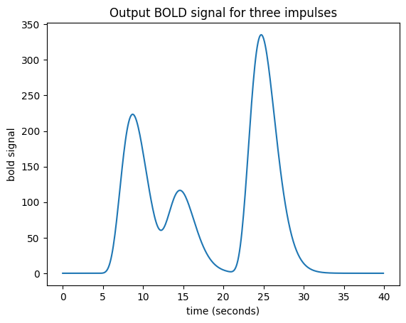
Maybe I can also make the assumption that the response to an impulse will be exactly the same over time. The response to any given impulse at time 10 will be the same as the response to the same impulse at time 4 or at time 30.

In that case my job is still simple. For the impulse amplitude 2 at time == 4, I add the HRF shifted to start at time == 4, and scaled by 2. To that result I then add the HRF shifted to time == 10 and scaled by 1. Finally, I further add the HRF shifted to time == 20 and scaled by 3:

bold_signal = np.zeros(n_time_points)
bold_signal[i_time_4:i_time_4 + n_hrf_points] = hrf_signal * 2
bold_signal[i_time_10:i_time_10 + n_hrf_points] += hrf_signal * 1
bold_signal[i_time_20:i_time_20 + n_hrf_points] += hrf_signal * 3
plt.plot(times, bold_signal)
plt.xlabel('time (seconds)')
plt.ylabel('bold signal')
plt.title('Output BOLD signal for three impulses')

Text(0.5, 1.0, 'Output BOLD signal for three impulses')

At the moment, an impulse is an event that lasts for just one time point. In our case, the time vector (times in the code above) has one point for every 0.1 seconds (10 time points per second).

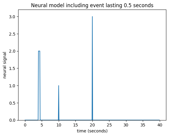
What happens if an event lasts for 0.5 seconds? Maybe I can assume that an event lasting 0.5 seconds has exactly the same effect as 5 impulses 0.1 seconds apart:

neural_signal[i_time_4:i_time_4 + 5] = 2
plt.plot(times, neural_signal)
plt.xlabel('time (seconds)')
plt.ylabel('neural signal')
plt.ylim(0, 3.2)
plt.title('Neural model including event lasting 0.5 seconds')

Text(0.5, 1.0, 'Neural model including event lasting 0.5 seconds')

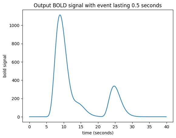
Now I need to add a new shifted HRF for the impulse corresponding to time == 4, and for time == 4.1 and so on until time == 4.4:

bold_signal = np.zeros(n_time_points)
for i in range(5):
    bold_signal[i_time_4 + i:i_time_4  + i + n_hrf_points] += hrf_signal * 2
bold_signal[i_time_10:i_time_10 + n_hrf_points] += hrf_signal * 1
bold_signal[i_time_20:i_time_20 + n_hrf_points] += hrf_signal * 3
plt.plot(times, bold_signal)
plt.xlabel('time (seconds)')
plt.ylabel('bold signal')
plt.title('Output BOLD signal with event lasting 0.5 seconds')

Text(0.5, 1.0, 'Output BOLD signal with event lasting 0.5 seconds')

Working out an algorithm

Now we have a general algorithm for making our output hemodynamic signal from our input neural signal:

1. Start with an output vector that is a vector of zeros;

2. For each index \(i\) in the input vector (the neural signal):

   1. Prepare a shifted copy of the HRF vector, starting at \(i\). Call this the shifted HRF vector;

   2. Multiply the shifted HRF vector by the value in the input at index \(i\), to give the shifted, scaled HRF vector;

   3. Add the shifted scaled HRF vector to the output.

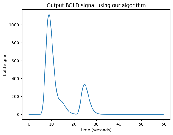
There is a little problem with our algorithm — the length of the output vector.

Imagine that our input (neural) vector is N time points long. Say the original HRF vector is M time points long.

In our algorithm, when the iteration gets to the last index of the input vector (\(i = N-1\)), the shifted scaled HRF vector will, as ever, be M points long. If the output vector is the same length as the input vector, we can add only the first point of the new scaled HRF vector to the last point of the output vector, but all the subsequent values of the scaled HRF vector extend off the end of the output vector and have no corresponding index in the output. The way to solve this is to extend the output vector by the necessary M-1 points. Now we can do our algorithm in code.

N = n_time_points
M = n_hrf_points
bold_signal = np.zeros(N + M - 1)  # adding the tail
for i in range(N):
    input_value = neural_signal[i]
    # Adding the shifted, scaled HRF
    bold_signal[i : i + n_hrf_points] += hrf_signal * input_value
# We have to extend 'times' to deal with more points in 'bold_signal'
extra_times = np.arange(n_hrf_points - 1) * 0.1 + 40
times_and_tail = np.concatenate((times, extra_times))
plt.plot(times_and_tail, bold_signal)
plt.xlabel('time (seconds)')
plt.ylabel('bold signal')
plt.title('Output BOLD signal using our algorithm')

Text(0.5, 1.0, 'Output BOLD signal using our algorithm')

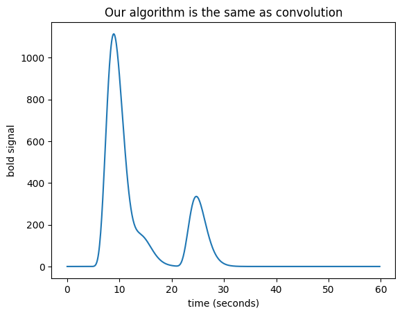
We have convolution

We now have — convolution. Here’s the same thing using the numpy convolve function:

bold_signal = np.convolve(neural_signal, hrf_signal)
plt.plot(times_and_tail, bold_signal)
plt.xlabel('time (seconds)')
plt.ylabel('bold signal')
plt.title('Our algorithm is the same as convolution')

Text(0.5, 1.0, 'Our algorithm is the same as convolution')

For more detail and background, see convolution with matrices