Convolution with matrices

import numpy as np
import matplotlib.pyplot as plt

This page follows on directly from the convolution page. It builds on some simple 2D arrays (matrices) to the formal mathematical definition of convolution. This page may be useful to you as more background and deeper understanding. We often do implement convolution with matrices, so the matrix formulation here will be useful for when you see this in code, or you are implementing convolution yourself.

Neural and hemodynamic prediction

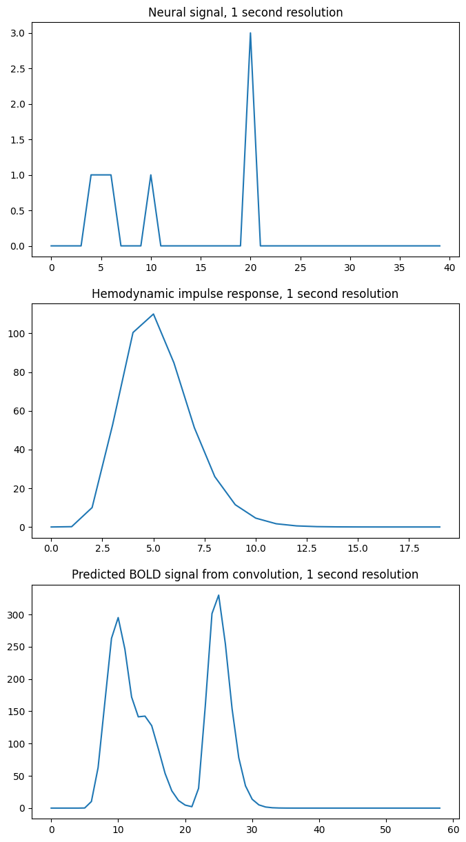
You will remember, from that page, that we were looking at neural prediction models, with spikes or blocks of “on” activity, and plateaus of “off” activity.

We were then convolving the neural activity with our estimate of the effect on blood flow of a instantaneous spike or “impulse” of neural activity. This estimate is the Hemodynamic Response Function (HRF).

From that page, we recover our example HRF.

def hrf(t):
    "A hemodynamic response function"
    return t ** 8.6 * np.exp(-t / 0.547)

In the main convolution page, we used very short time bins of 0.1 seconds to define whether the neural response was “on” or not. Thus, the shortest impulse we allow for is 0.1 seconds.

For what follows, it is a bit easier to see what is going on with a lower time resolution — say one time point per second. We will make the first event last 3 seconds:

times = np.arange(0, 40)  # One time point per second
n_time_points = len(times)
neural_signal = np.zeros(n_time_points)

neural_signal[4:7] = 1  # A 3 second event
neural_signal[10] = 1
neural_signal[20] = 3

hrf_times = np.arange(20)
hrf_signal = hrf(hrf_times)  # The HRF at one second time resolution
n_hrf_points = len(hrf_signal)

bold_signal = np.convolve(neural_signal, hrf_signal)

times_and_tail = np.arange(n_time_points + n_hrf_points - 1)

fig, axes = plt.subplots(3, 1, figsize=(8, 15))
axes[0].plot(times, neural_signal)
axes[0].set_title('Neural signal, 1 second resolution')
axes[1].plot(hrf_times, hrf_signal)
axes[1].set_title('Hemodynamic impulse response, 1 second resolution')
axes[2].plot(times_and_tail, bold_signal)
axes[2].set_title('Predicted BOLD signal from convolution, 1 second resolution')

Text(0.5, 1.0, 'Predicted BOLD signal from convolution, 1 second resolution')

Our algorithm, which turned out to give convolution, had us add a shifted, scaled version of the HRF to the output, for every index. Here is the algorithm from the convolution page:

1. Start with an output vector that is a vector of zeros;

2. For each index \(i\) in the input vector (the neural signal):

   1. Prepare a shifted copy of the HRF vector, starting at \(i\). Call this the shifted HRF vector;

   2. Multiply the shifted HRF vector by the value in the input at index \(i\), to give the shifted, scaled HRF vector;

   3. Add the shifted scaled HRF vector to the output.

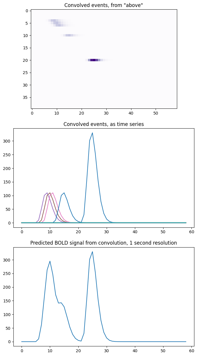
Now imagine that, instead of adding the shifted scaled HRF to the output vector, we store each shifted scaled HRF as a row in an array, that has one row for each index in the input vector. Then we can get the same output vector as before by taking the sum across the columns of this array:

N = n_time_points
M = n_hrf_points
shifted_scaled_hrfs = np.zeros((N, N + M - 1))
for i in range(N):
    input_value = neural_signal[i]
    # Storing the shifted, scaled HRF
    shifted_scaled_hrfs[i, i : i + n_hrf_points] = hrf_signal * input_value
bold_signal_again = np.sum(shifted_scaled_hrfs, axis=0)

# We check that the result is almost exactly the same
# (allowing for tiny differences due to the order of +, * operations)
import numpy.testing as npt
npt.assert_almost_equal(bold_signal, bold_signal_again)

To visualize this, let’s look at the shifted_scaled_hrfs matrix as an image where darker colors indicate higher values. We can then look at it as a collection of time series, and see how it adds to produce our expected BOLD signal:

fig, axes = plt.subplots(3, 1, figsize=(8, 15))
axes[0].imshow(shifted_scaled_hrfs, cmap='Purples')
axes[0].set_title('Convolved events, from "above"')
axes[1].plot(times_and_tail, shifted_scaled_hrfs.T)
axes[1].set_title('Convolved events, as time series')
axes[2].plot(times_and_tail, bold_signal_again)
axes[2].set_title('Predicted BOLD signal from convolution, 1 second resolution')

Text(0.5, 1.0, 'Predicted BOLD signal from convolution, 1 second resolution')

We can also do exactly the same operation by first making an array with the shifted HRFs, without scaling, and then multiplying each row by the corresponding input value, before doing the sum. Here we are doing the shifting first, and then the scaling, and then the sum. It all adds up to the same operation:

# First we make the shifted HRFs
shifted_hrfs = np.zeros((N, N + M - 1))
for i in range(N):
    # Storing the shifted HRF without scaling
    shifted_hrfs[i, i : i + n_hrf_points] = hrf_signal
# Then do the scaling
shifted_scaled_hrfs = np.zeros((N, N + M - 1))
for i in range(N):
    input_value = neural_signal[i]
    # Scaling the stored HRF by the input value
    shifted_scaled_hrfs[i, :] = shifted_hrfs[i, :] * input_value
# Then the sum
bold_signal_again = np.sum(shifted_scaled_hrfs, axis=0)
# This gives the same result, once again
npt.assert_almost_equal(bold_signal, bold_signal_again)

The shifted_hrfs array looks like this as an image:

plt.imshow(shifted_hrfs, cmap='Purples')

<matplotlib.image.AxesImage at 0x7fed1ca8b130>

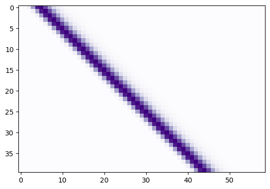
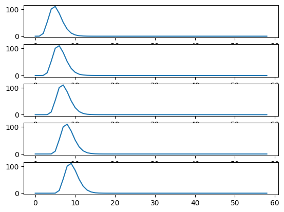
Each new row of shifted_hrfs corresponds to the HRF, shifted by one more column to the right:

fig, axes = plt.subplots(5, 1)
for row_no in range(5):
    axes[row_no].plot(shifted_hrfs[row_no, :])

Now remember how matrix multiplication works:

\[\begin{split} \begin{pmatrix} xa + yb + zc \\ xd + ye + zf \end{pmatrix} = \begin{pmatrix} x & y & z \end{pmatrix} \begin{pmatrix} a & d \\ b & e \\ c & f \end{pmatrix} \end{split}\]

Now let us make our input neural vector into a 1 by N row vector. If we matrix multiply this vector onto the shifted_hrfs array (matrix), then we do the scaling of the HRFs and the sum operation, all in one go. Like this:

def as_row_vector(v):
    " Convert 1D vector to row vector "
    return v.reshape((1, -1))

neural_vector = as_row_vector(neural_signal)
# The scaling and summing by the magic of matrix multiplication
bold_signal_again = neural_vector @ shifted_hrfs
# This gives the same result as previously, yet one more time
npt.assert_almost_equal(as_row_vector(bold_signal), bold_signal_again)

The matrix transpose rule says \((A B)^T = B^T A^T\) where \(A^T\) is the transpose of matrix \(A\). So we could also do this exact same operation by doing a matrix multiply of the transpose of shifted_hrfs onto the neural_signal as a column vector:

bold_signal_again = shifted_hrfs.T @ neural_vector.T
# Exactly the same, but transposed
npt.assert_almost_equal(as_row_vector(bold_signal), bold_signal_again.T)

In this last formulation, the shifted_hrfs matrix is the convolution matrix, in that (as we have just shown) you can apply the convolution of the HRF by matrix multiplying onto an input vector.

Convolution is like cross-correlation with the reversed HRF

We are now ready to show something slightly odd that arises from the way that convolution works.

Consider index \(i\) in the input (neural) vector. Let’s say \(i = 25\). We want to get value index \(i\) in the output (hemodynamic vector). What do we need to do?

Looking at our non-transposed matrix formulation, we see that value \(i\) in the output is the matrix multiplication of the neural signal (row vector) by column \(i\) in shifted_hrfs. Here is a plot of column 25 in shifted_hrfs:

plt.plot(shifted_hrfs[:, 25])

[<matplotlib.lines.Line2D at 0x7fed1c26cac0>]

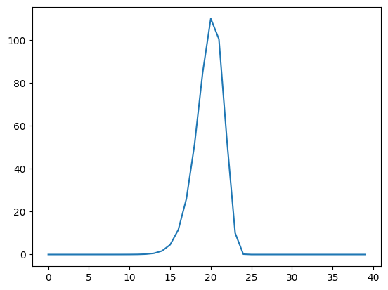
The column contains a reversed copy of the HRF signal, where the first value from the original HRF signal is at index 25 (\(i\)), the second value is at index 24 (\(i - 1\)) and so on back to index 25 - 20 = 5. The reversed HRF follows from the way we constructed the rows of the original matrix. Each new HRF row was shifted across by one column, therefore, reading up the columns from the diagonals, will also give you the HRF shape.

Let us rephrase the matrix multiplication that gives us the value at index \(i\) in the output vector. Call the neural input vector \(\mathbf{n}\) with values \(n_0, n_1 ... n_{N-1}\). Call the shifted_hrfs array \(\mathbf{S}\) with \(N\) rows and \(N + M - 1\) columns. \(\mathbf{S}_{:,i}\) is column \(i\) in \(\mathbf{S}\).

So, the output value \(o_i\) is given by the matrix multiplication of row \(\mathbf{n}\) onto column \(\mathbf{S}_{:,i}\). The matrix multiplication (dot product) gives us the usual sum of products as the output:

\[ o_i = \sum_{j=0}^{N-1}{n_j S_{j,i}} \]

The formula above describes what is happening in the matrix multiplication in this piece of code:

i = 25
bold_i = neural_vector @ shifted_hrfs[:, i]

npt.assert_almost_equal(bold_i, bold_signal[i])

Can we simplify the formula without using the shifted_hrfs \(\mathbf{S}\) matrix? We saw above that column \(i\) in shifted_hrfs contains a reversed HRF, starting at index \(i\) and going backwards towards index 0.

The 1-second resolution HRF is our array hrf_signal. So shifted_hrfs[i, i] contains hrf_signal[0], shifted_hrfs[i-1, i] contains hrf_signal[1] and so on. In general, for any index \(j\) into shifted_hrfs[:, i], shifted_hrfs[j, i] == hrf_signal[i-j] (assuming we return zero for any hrf_signal[i-j] where i-j is outside the bounds of the vector, with i-j < 0 or \(\geq\) M).

Realizing this, we can replace \(\mathbf{S}_{:,i}\) in our equation above. Call our hrf_signal vector \(\mathbf{h}\) with values \(h_0, h_1, ... h_{M-1}\). Then:

\[ o_i = \sum_{j=0}^{N-1}{n_j h_{i-j}} \]

This is the sum of the {products of the elements of \(\mathbf{n}\) with the matching elements from the [reversed HRF vector \(\mathbf{h}\), shifted by \(i\) elements]}.

The mathematical definition for convolution

This brings us to the abstract definition of convolution for continuous functions.

In general, call the continuous input a function \(f\). In our case the input signal is the neuronal model, that is a function of time. This is the continuous generalization of the vector \(\mathbf{n}\) in our discrete model. The continuous function to convolve with is \(g\). In our case \(g\) is the HRF, also a function of time. \(g\) is the generalized continuous version of the vector \(\mathbf{h}\) in the previous section. The convolution of \(f\) and \(g\) is often written \((f * g)\) and for any given \(t\) is defined as:

\[ (f * g )(t) \stackrel{\mathrm{def}}{=}\ \int_{-\infty}^\infty f(\tau)\, g(t - \tau)\, d\tau \]

As you can see, and as we have already discovered in the discrete case, the convolution is the integral of the product of the two functions as the second function \(g\) is reversed and shifted.

See : the wikipedia convolution definition section for more discussion.