Registration with dipy#
Dipy is a Python package for diffusion imaging.
Install in the usual way from the terminal:
pip3 install --user dipy
It has general image registration algorithms, including affine and non-linear registration.
These are based on the model and algorithms implemented in the ANTS toolbox. ANTS is written in C++.
Python is an excellent language to work in for this problem because Python code is easier for most scientists to read than C++. Dipy uses an optimized, compiled Python / C fusion language called Cython, that allows us to mix Python code and C-like code, to give speed of execution close to that of hand-written C code.
This page is closely based on the 3D registration tutorials in the Dipy documentation:
# Set up our usual routines and configuration
import numpy as np
np.set_printoptions(precision=4, suppress=True)

import matplotlib.pyplot as plt
plt.rcParams['image.cmap'] = 'gray'

import nibabel as nib

import nipraxis
Affine registration#
Import the Dipy routines we are going to need:
from dipy.viz import regtools
from dipy.align.imaffine import (AffineMap,
                                 MutualInformationMetric,
                                 AffineRegistration)
from dipy.align.transforms import (TranslationTransform3D,
                                   RigidTransform3D,
                                   AffineTransform3D)
/opt/hostedtoolcache/Python/3.10.13/x64/lib/python3.10/site-packages/tqdm/auto.py:21: TqdmWarning: IProgress not found. Please update jupyter and ipywidgets. See https://ipywidgets.readthedocs.io/en/stable/user_install.html
  from .autonotebook import tqdm as notebook_tqdm
Next we load the subject structural image and the template image. These images have already had all voxels outside the brain set to zero. For the individual subject image, the OpenFMRI project ran the FSL Brain Extraction Tool on the image before uploading to the OpenFMRI website. The template comes with an image defining in-brain voxels. The registration works better on images for which we have masked out the skull and face.
# Masked structural
masked_subj_fname = nipraxis.fetch_file('ds114_sub009_highres_brain_222.nii')
masked_subj_fname
Downloading file 'ds114_sub009_highres_brain_222.nii' from 'https://raw.githubusercontent.com/nipraxis/nipraxis-data/0.5/ds114_sub009_highres_brain_222.nii' to '/home/runner/.cache/nipraxis/0.5'.
'/home/runner/.cache/nipraxis/0.5/ds114_sub009_highres_brain_222.nii'
# Masked template
masked_template_fname = nipraxis.fetch_file(
    'mni_icbm152_t1_tal_nlin_asym_09a_masked_222.nii')
masked_template_fname
Downloading file 'mni_icbm152_t1_tal_nlin_asym_09a_masked_222.nii' from 'https://raw.githubusercontent.com/nipraxis/nipraxis-data/0.5/mni_icbm152_t1_tal_nlin_asym_09a_masked_222.nii' to '/home/runner/.cache/nipraxis/0.5'.
'/home/runner/.cache/nipraxis/0.5/mni_icbm152_t1_tal_nlin_asym_09a_masked_222.nii'
moving_img = nib.load(masked_subj_fname)
template_img = nib.load(masked_template_fname)
Dipy works on the image data arrays. It also needs the affine arrays of each of the images:
moving_data = moving_img.get_fdata()
moving_affine = moving_img.affine
template_data = template_img.get_fdata()
template_affine = template_img.affine
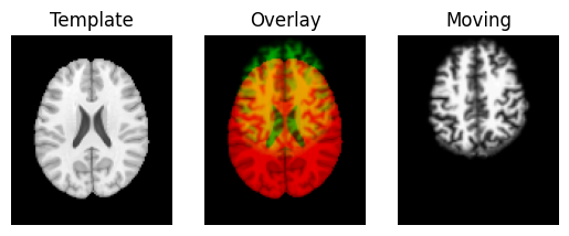
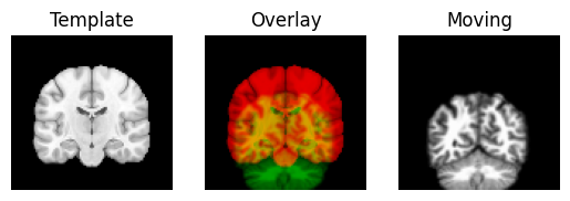
We use the nice Dipy routines to show the spatial correspondence of the images, as recorded in the affines.
identity = np.eye(4)
affine_map = AffineMap(identity,
                       template_data.shape, template_affine,
                       moving_data.shape, moving_affine)
resampled = affine_map.transform(moving_data)
regtools.overlay_slices(template_data, resampled, None, 0,
                        "Template", "Moving")
regtools.overlay_slices(template_data, resampled, None, 1,
                        "Template", "Moving")
regtools.overlay_slices(template_data, resampled, None, 2,
                        "Template", "Moving")


Next we define an affine registration, by giving a few standard parameters. See the Dipy registration tutorial for the details of what these parameters mean:
# The mismatch metric
nbins = 32
sampling_prop = None
metric = MutualInformationMetric(nbins, sampling_prop)
# The optimization strategy
level_iters = [10, 10, 5]
sigmas = [3.0, 1.0, 0.0]
factors = [4, 2, 1]
We set up the registration object, ready to do the registration:
affreg = AffineRegistration(metric=metric,
                            level_iters=level_iters,
                            sigmas=sigmas,
                            factors=factors)
First we optimize the translations. We do the translations first to get these in the ballpark. After that we will estimate translations and rotations together, using the estimated translations as a starting point. Last we will use the translations and rotations as a starting point for a full affine registration.
transform = TranslationTransform3D()
params0 = None
translation = affreg.optimize(template_data, moving_data, transform, params0,
                              template_affine, moving_affine)
Optimizing level 2 [max iter: 10]
Optimizing level 1 [max iter: 10]
Optimizing level 0 [max iter: 5]
We now have our estimated translations.
translation.affine
array([[  1.    ,   0.    ,   0.    ,  -1.8557],
       [  0.    ,   1.    ,   0.    ,  39.6567],
       [  0.    ,   0.    ,   1.    , -22.0912],
       [  0.    ,   0.    ,   0.    ,   1.    ]])
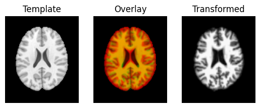
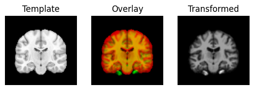
The visualization tool now shows the images overlay much better than they did before:
transformed = translation.transform(moving_data)
regtools.overlay_slices(template_data, transformed, None, 0,
                        "Template", "Transformed")
regtools.overlay_slices(template_data, transformed, None, 1,
                        "Template", "Transformed")
regtools.overlay_slices(template_data, transformed, None, 2,
                        "Template", "Transformed")


Next we use the estimated translations as a starting point to optimize a rigid-body transform. A rigid-body transform is a transform that does not change the shape of the object. It allows only translations and rotations.
transform = RigidTransform3D()
rigid = affreg.optimize(template_data, moving_data, transform, params0,
                        template_affine, moving_affine,
                        starting_affine=translation.affine)
Optimizing level 2 [max iter: 10]
Optimizing level 1 [max iter: 10]
Optimizing level 0 [max iter: 5]
rigid.affine
array([[  0.9995,  -0.0269,  -0.0166,  -2.3604],
       [  0.0265,   0.9993,  -0.0268,  40.0467],
       [  0.0173,   0.0264,   0.9995, -21.0786],
       [  0.    ,   0.    ,   0.    ,   1.    ]])
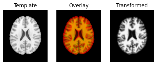
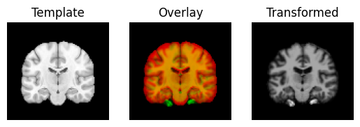
The estimated rotations are small, so they don’t make much difference to the overlay of the image.
transformed = rigid.transform(moving_data)
regtools.overlay_slices(template_data, transformed, None, 0,
                        "Template", "Transformed")
regtools.overlay_slices(template_data, transformed, None, 1,
                        "Template", "Transformed")
regtools.overlay_slices(template_data, transformed, None, 2,
                        "Template", "Transformed")


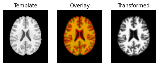
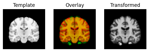
Last, we do a full affine registration, using the rigid body estimate as a starting point.
transform = AffineTransform3D()
# Bump up the iterations to get an more exact fit
affreg.level_iters = [1000, 1000, 100]
affine = affreg.optimize(template_data, moving_data, transform, params0,
                         template_affine, moving_affine,
                         starting_affine=rigid.affine)
Optimizing level 2 [max iter: 1000]
Optimizing level 1 [max iter: 1000]
Optimizing level 0 [max iter: 100]
affine.affine
array([[  0.935 ,  -0.0268,   0.0009,  -2.1728],
       [  0.0438,   0.9553,  -0.0418,  39.0283],
       [  0.0117,   0.0239,   0.8903, -19.107 ],
       [  0.    ,   0.    ,   0.    ,   1.    ]])
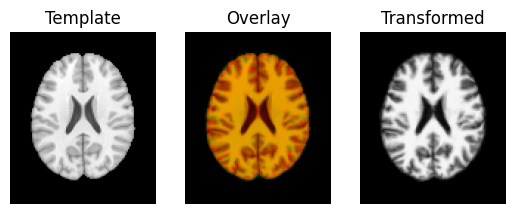
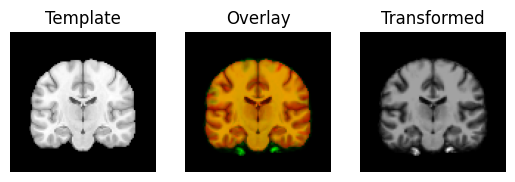
transformed = affine.transform(moving_data)
regtools.overlay_slices(template_data, transformed, None, 0,
                        "Template", "Transformed")
regtools.overlay_slices(template_data, transformed, None, 1,
                        "Template", "Transformed")
regtools.overlay_slices(template_data, transformed, None, 2,
                        "Template", "Transformed")


Non-linear registration#
from dipy.align.imwarp import SymmetricDiffeomorphicRegistration
from dipy.align.imwarp import DiffeomorphicMap
from dipy.align.metrics import CCMetric
# The mismatch metric
metric = CCMetric(3)
# The optimization strategy:
level_iters = [10, 10, 5]
# Registration object
sdr = SymmetricDiffeomorphicRegistration(metric, level_iters)
Do the registration:
mapping = sdr.optimize(template_data, moving_data, template_affine,
                       moving_affine, affine.affine)
Resample using the new parameters:
warped_moving = mapping.transform(moving_data)
Display the transformed (warped) image:
regtools.overlay_slices(template_data, warped_moving, None, 0,
                        "Template", "Transformed")
regtools.overlay_slices(template_data, warped_moving, None, 1,
                        "Template", "Transformed")
regtools.overlay_slices(template_data, warped_moving, None, 2,
                        "Template", "Transformed")
