Convolving with the hemodyamic response function

Start with our usual imports:

import numpy as np
import matplotlib.pyplot as plt

Making a hemodynamic response function

We will start by making a function that returns an estimate of the blood flow signal at any time \(t\) after the onset of a neural impulse.

We could use measured data to do this, from data like this paper, with the problem that the data has some noise that we do not want to preserve. Another way, that we follow here, is to construct a function from some useful mathematical curves that gives values that are of a very similar shape to the measured response over time.

Using scipy

Scipy is a large library of scientific routines that builds on top of numpy.

You can think of numpy as being a subset of MATLAB, and numpy + scipy as being as being roughly equivalent to MATLAB plus the MATLAB toolboxes.

Scipy has many sub-packages, for doing things like reading MATLAB .mat files (scipy.io) or working with sparse matrices (scipy.sparse). We are going to be using the functions and objects for working with statistical distributions in scipy.stats:

import scipy.stats

scipy.stats contains objects for working with many different distributions. We are going to be working with scipy.stats.gamma, which implements the gamma distribution.

from scipy.stats import gamma

In particular we are interested in the probability density function (PDF) of the gamma distribution.

Because this is a function, we need to pass it an array of values at which it will evaluate.

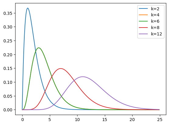
We can also pass various parameters which change the shape, location and width of the gamma PDF. The most important is the first parameter (after the input array) known as the shape parameter (\(k\) in the wikipedia page on gamma distributions).

First we chose some x values at which to sample from the gamma PDF:

x = np.arange(0, 25, 0.1)

Next we plot the gamma PDF for shape values of 2, 4, 6, 8, 12.

plt.plot(x, gamma.pdf(x, 2), label='k=2')
plt.plot(x, gamma.pdf(x, 4), label='k=4')
plt.plot(x, gamma.pdf(x, 4), label='k=6')
plt.plot(x, gamma.pdf(x, 8), label='k=8')
plt.plot(x, gamma.pdf(x, 12), label='k=12')
plt.legend()

<matplotlib.legend.Legend at 0x7f18357e2560>

Constructing a hemodynamic response function

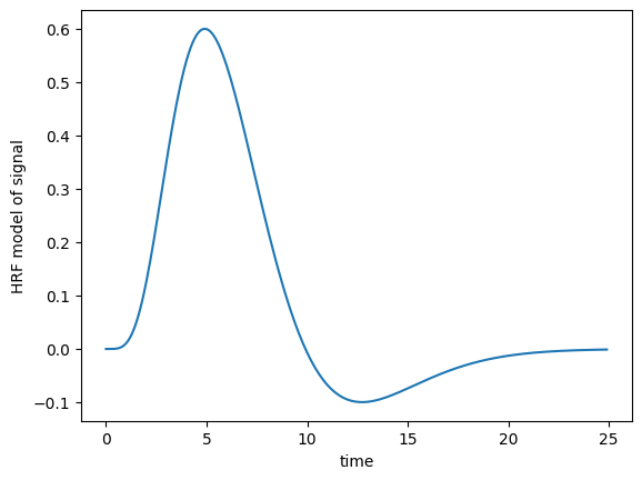
We can use these gamma functions to construct a continuous function that is close to the hemodynamic response we observe for a single brief event in the brain.

Our function will accept an array that gives the times we want to calculate the HRF for, and returns the values of the HRF for those times. We will assume that the true HRF starts at zero, and gets to zero sometime before 35 seconds.

We’re going to try using the sum of two gamma distribution probability density functions.

Here is one example of such a function:

def hrf(times):
    """ Return values for HRF at given times """
    # Gamma pdf for the peak
    peak_values = gamma.pdf(times, 6)
    # Gamma pdf for the undershoot
    undershoot_values = gamma.pdf(times, 12)
    # Combine them
    values = peak_values - 0.35 * undershoot_values
    # Scale max to 0.6
    return values / np.max(values) * 0.6

plt.plot(x, hrf(x))
plt.xlabel('time')
plt.ylabel('HRF model of signal')

Text(0, 0.5, 'HRF model of signal')

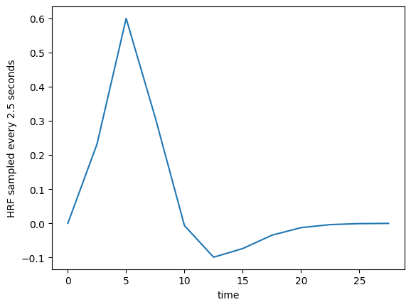
We can sample from the function, to get the estimates at the times of our TRs. Remember, the TR is 2.5 for our example data, meaning the scans were 2.5 seconds apart.

TR = 2.5
tr_times = np.arange(0, 30, TR)
hrf_at_trs = hrf(tr_times)
print(len(hrf_at_trs))
plt.plot(tr_times, hrf_at_trs)
plt.xlabel('time')
plt.ylabel('HRF sampled every 2.5 seconds')

12

Text(0, 0.5, 'HRF sampled every 2.5 seconds')

We can use this to convolve our neural (on-off) prediction. This will give us a hemodynamic prediction, under the linear-time-invariant assumptions of the convolution.

First we get the condition file:

# Load the function to fetch the data file we need.
import nipraxis
# Fetch the data file.
cond_fname = nipraxis.fetch_file('ds114_sub009_t2r1_cond.txt')
# Show the file name of the fetched data.
cond_fname

Downloading file 'ds114_sub009_t2r1_cond.txt' from 'https://raw.githubusercontent.com/nipraxis/nipraxis-data/0.5/ds114_sub009_t2r1_cond.txt' to '/home/runner/.cache/nipraxis/0.5'.

'/home/runner/.cache/nipraxis/0.5/ds114_sub009_t2r1_cond.txt'

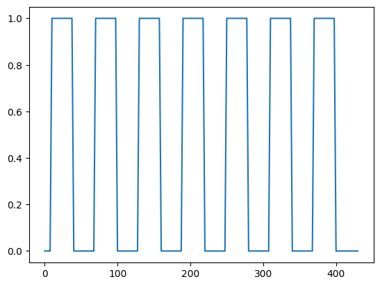
Next we using a version of the stimulus.py file we worked on earlier, to convert the onsets in the file, to neural time-courses.

from nipraxis.stimuli import events2neural
n_vols = 173
neural_prediction = events2neural(cond_fname, TR, n_vols)
all_tr_times = np.arange(173) * TR
plt.plot(all_tr_times, neural_prediction)

[<matplotlib.lines.Line2D at 0x7f1832fedc00>]

When we convolve, the output is length N + M-1, where N is the number of values in the vector we convolved, and M is the length of the convolution kernel (hrf_at_trs in our case). For a reminder of why this is, see the tutorial on convolution.

convolved = np.convolve(neural_prediction, hrf_at_trs)
N = len(neural_prediction)  # M == n_vols == 173
M = len(hrf_at_trs)  # M == 12
len(convolved) == N + M - 1

True

This is because of the HRF convolution kernel falling off the end of the input vector. The value at index 172 in the new vector refers to time 172 * 2.5 = 430.0 seconds, and value at index 173 refers to time 432.5 seconds, which is just after the end of the scanning run. To retain only the values in the new hemodynamic vector that refer to times up to (and including) 430s, we can just drop the last len(hrf_at_trs) - 1 == M - 1 values:

n_to_remove = len(hrf_at_trs) - 1
convolved = convolved[:-n_to_remove]

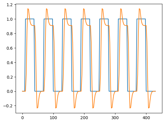
plt.plot(all_tr_times, neural_prediction)
plt.plot(all_tr_times, convolved)

[<matplotlib.lines.Line2D at 0x7f1832e666e0>]

For our future use, might want to save our convolved time course to a numpy text file:

# Save the convolved time course to 6 decimal point precision
np.savetxt('ds114_sub009_t2r1_conv.txt', convolved, fmt='%2.6f')
back = np.loadtxt('ds114_sub009_t2r1_conv.txt')
# Check written data is within 0.000001 of original
np.allclose(convolved, back, atol=1e-6)

True

There is a copy of this saved file in the Nipraxis data collection, that we will use later.