Modeling a single voxel

Modeling a single voxel#

The voxel regression page has a worked example of applying simple regression) on a single voxel.

This page runs the same calculations, but using the General Linear Model notation and matrix calculations.

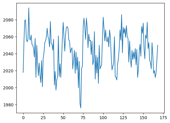
Let’s get that same voxel time course back again:

import numpy as np
import matplotlib.pyplot as plt
import nibabel as nib
# Only show 6 decimals when printing
np.set_printoptions(precision=6)

# Load the function to fetch the data file we need.
import nipraxis
# Fetch the data file.
data_fname = nipraxis.fetch_file('ds114_sub009_t2r1.nii')
img = nib.load(data_fname)
data = img.get_fdata()
# Knock off the first four volumes (to avoid artefact).
data = data[..., 4:]
# Get the voxel time course of interest.
voxel_time_course = data[42, 32, 19]
plt.plot(voxel_time_course)

[<matplotlib.lines.Line2D at 0x7f557836cbe0>]

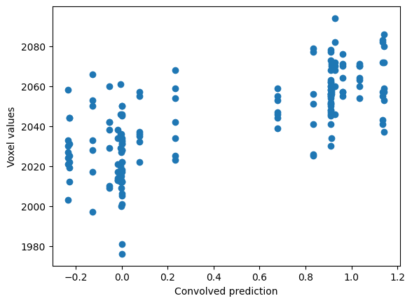
_images/e43d77989eb6969e3172bedf3f22795c38b314f2472a86de28e3fe1a0c519617.png

Load the convolved time course, and plot the voxel values against the convolved regressor:

tc_fname = nipraxis.fetch_file('ds114_sub009_t2r1_conv.txt')
# Show the file name of the fetched data.
convolved = np.loadtxt(tc_fname)
# Knock off first 4 elements to match data.
convolved = convolved[4:]
# Plot.
plt.scatter(convolved, voxel_time_course)
plt.xlabel('Convolved prediction')
plt.ylabel('Voxel values')

Downloading file 'ds114_sub009_t2r1_conv.txt' from 'https://raw.githubusercontent.com/nipraxis/nipraxis-data/0.5/ds114_sub009_t2r1_conv.txt' to '/home/runner/.cache/nipraxis/0.5'.

Text(0, 0.5, 'Voxel values')

_images/399b877b6133629133f5ccc019f4889be24d936b9434c0e9316256c530effb91.png

As you remember, we apply the GLM by first preparing a design matrix, that has one column corresponding for each parameter in the model.

In our case we have two parameters, the slope and the intercept.

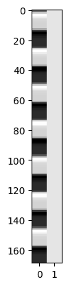
First we make our design matrix. It has a column for the convolved regressor, and a column of ones:

N = len(convolved)
X = np.ones((N, 2))
X[:, 0] = convolved
plt.imshow(X, cmap='gray', aspect=0.1, interpolation='none')

<matplotlib.image.AxesImage at 0x7f55783b6830>

_images/12ff4e781d96313abc1d7a8db0e08a719fbb1aaaacd3191c25140023913622ff.png

Our model is:

\vec{y} = X \vec{β} + \vec{ε}

We can get our least mean squared error (MSE) parameter estimates for $\vec{β}$ with:

\hat{\vec{β}} = X^{+} y

where $X^{+}$ is the pseudoinverse of $X$ . When $X$ is invertible, the pseudoinverse is given by:

X^{+} = (X^{T} X)^{- 1} X^{T}

Let’s calculate the pseudoinverse for our design:

import numpy.linalg as npl
Xp = npl.pinv(X)
Xp.shape

(2, 169)

We calculate $\hat{\vec{β}}$ :

beta_hat = Xp @ voxel_time_course
beta_hat

array([  31.185514, 2029.367689])

We can then calculate $\hat{\vec{y}}$ (also called the fitted data):

y_hat = X @ beta_hat

Finally, we may be interested to calculate the MSE of this model:

# Residuals are actual minus fitted.
e_vec = voxel_time_course - y_hat
mse = np.mean(e_vec ** 2)
mse

245.00339852605674

Notice that the $\hat{\vec{β}}$ parameters are the same as the slope and intercept from the Scipy calculation using linregress:

import scipy.stats as sps
sps.linregress(convolved, voxel_time_course)

LinregressResult(slope=31.18551366491453, intercept=2029.367689291584, rvalue=0.7044637722561978, pvalue=1.1832511547748845e-26, stderr=2.4312815394118448, intercept_stderr=1.634742742490283)