Three-dimensional arrays

Three-dimensional arrays#

# Our usual set-up
import numpy as np
import matplotlib.pyplot as plt

# Set 'gray' as the default colormap
plt.rcParams['image.cmap'] = 'gray'

# Display array values to 4 digits of precision
np.set_printoptions(precision=4, suppress=True)

So far we have seen one-dimensional and two-dimensional arrays. These are easy to think about, the one-dimensional array is like a row from a table or spreadsheet. A two-dimensional array has rows and columns, like a table or a spreadsheet.

A three-dimensional array takes a little bit more work to visualize, and get used to.

Two dimensions before three#

One way to think of three-dimensional arrays is as stacks of 2D arrays.

Here are a couple of two-dimensional arrays.

# make the first 2D array
first_1d = np.arange(10, 22)
first_2d = np.reshape(first_1d, (4, 3))

# show the first 2D array
first_2d

array([[10, 11, 12],
       [13, 14, 15],
       [16, 17, 18],
       [19, 20, 21]])

# make the second 2D array
second_1d = np.arange(100, 112)
second_2d = np.reshape(second_1d, (4, 3))

# show the second 2D array
second_2d

array([[100, 101, 102],
       [103, 104, 105],
       [106, 107, 108],
       [109, 110, 111]])

We can get rows from the 2D arrays by slicing with an index on the first dimension, thus:

# Third row, all the columns.
first_2d[2, :]

array([16, 17, 18])

Or, we can get columns by slicing with an index on the second dimension:

# All the rows, second column.
first_2d[:, 1]

array([11, 14, 17, 20])

These 2D arrays have four elements along the first dimension (axis), and three elements along the second dimension (axis).

first_2d.shape

(4, 3)

They therefore have 4 * 3 = 12 elements each. The np.prod function multiples all the elements in a sequence, so we can get the number of elements in an array with:

# 4 * 3
np.prod(first_2d.shape)

but there is even a short-cut way to get that:

first_2d.size

Three dimensions#

Here we make a three-dimensional array, by stacking the two 2D arrays together.

Let’s look again at the first_2d array:

first_2d

array([[10, 11, 12],
       [13, 14, 15],
       [16, 17, 18],
       [19, 20, 21]])

and the second_2d array:

second_2d

array([[100, 101, 102],
       [103, 104, 105],
       [106, 107, 108],
       [109, 110, 111]])

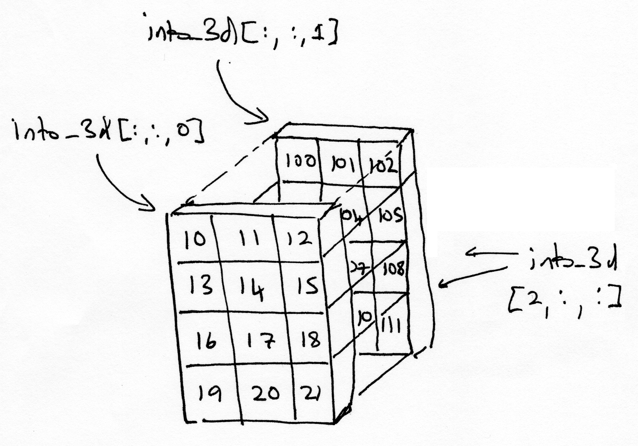
If you imagine the first_2d array and the second_2d array as flat physical objects, such as trays, then when we stack them, we will get the 3D array shown in the image below:

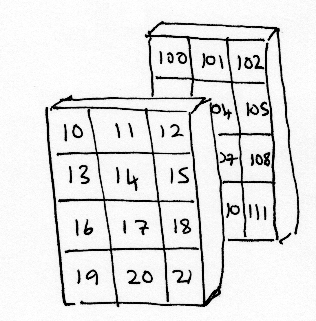
The object in the foreground of the image (with 10, 11, 12 on its topmost row) is the first plane of the 3D array, and contains the values from the first_2d array. The object in the background of the image (with 100, 101, 102 on its topmost row) is the second plane, and contains the values from the second_2d array.

We can use np.stack to stack the two 2D arrays into a 3D array. Here we want to stack over the third axis (axis=2):

# Make a 3D array by stacking the two 2D arrays.
into_3d = np.stack([first_2d, second_2d], axis=2)
# Show the result.  This display is not easy to read, see below for more.
into_3d

array([[[ 10, 100],
        [ 11, 101],
        [ 12, 102]],

       [[ 13, 103],
        [ 14, 104],
        [ 15, 105]],

       [[ 16, 106],
        [ 17, 107],
        [ 18, 108]],

       [[ 19, 109],
        [ 20, 110],
        [ 21, 111]]])

The 3D array, as Numpy shows it, might not have an obvious resemblance to the image of the two planes shown above, but bear with us.

The 3D array is of the right shape:

into_3d.shape

(4, 3, 2)

The shape can be read as “two planes, each with 4 rows and 3 columns”, which corresponds to what is shown in the image of the planes above.

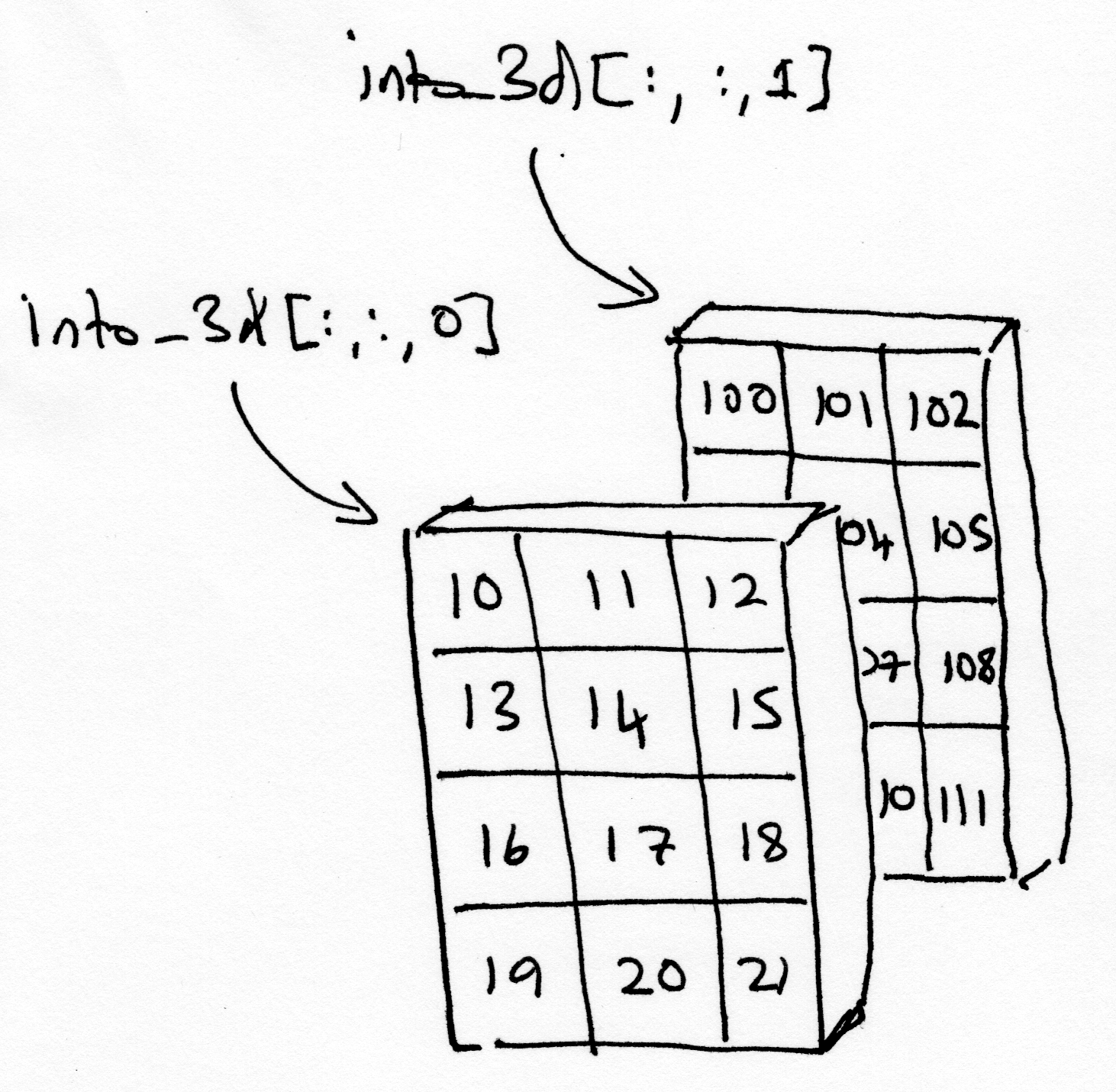
We can use indexing to fetch the component 2D planes back out of the 3D array.

There are three dimensions, so we can use three elements for indexing, separated by commas. The first element is for rows, the second for columns, and the third for planes.

# Fetch the first 2D plane.
# Read this as 'all rows, all columns of plane 0'
into_3d[:, :, 0]

array([[10, 11, 12],
       [13, 14, 15],
       [16, 17, 18],
       [19, 20, 21]])

# Fetch the second 2D plane.
# Read this as 'all rows, all columns of plane 1'
into_3d[:, :, 1]

array([[100, 101, 102],
       [103, 104, 105],
       [106, 107, 108],
       [109, 110, 111]])

You have already seen the output of the cell below. It is the way that Numpy shows us the contents of the into_3d array:

into_3d

array([[[ 10, 100],
        [ 11, 101],
        [ 12, 102]],

       [[ 13, 103],
        [ 14, 104],
        [ 15, 105]],

       [[ 16, 106],
        [ 17, 107],
        [ 18, 108]],

       [[ 19, 109],
        [ 20, 110],
        [ 21, 111]]])

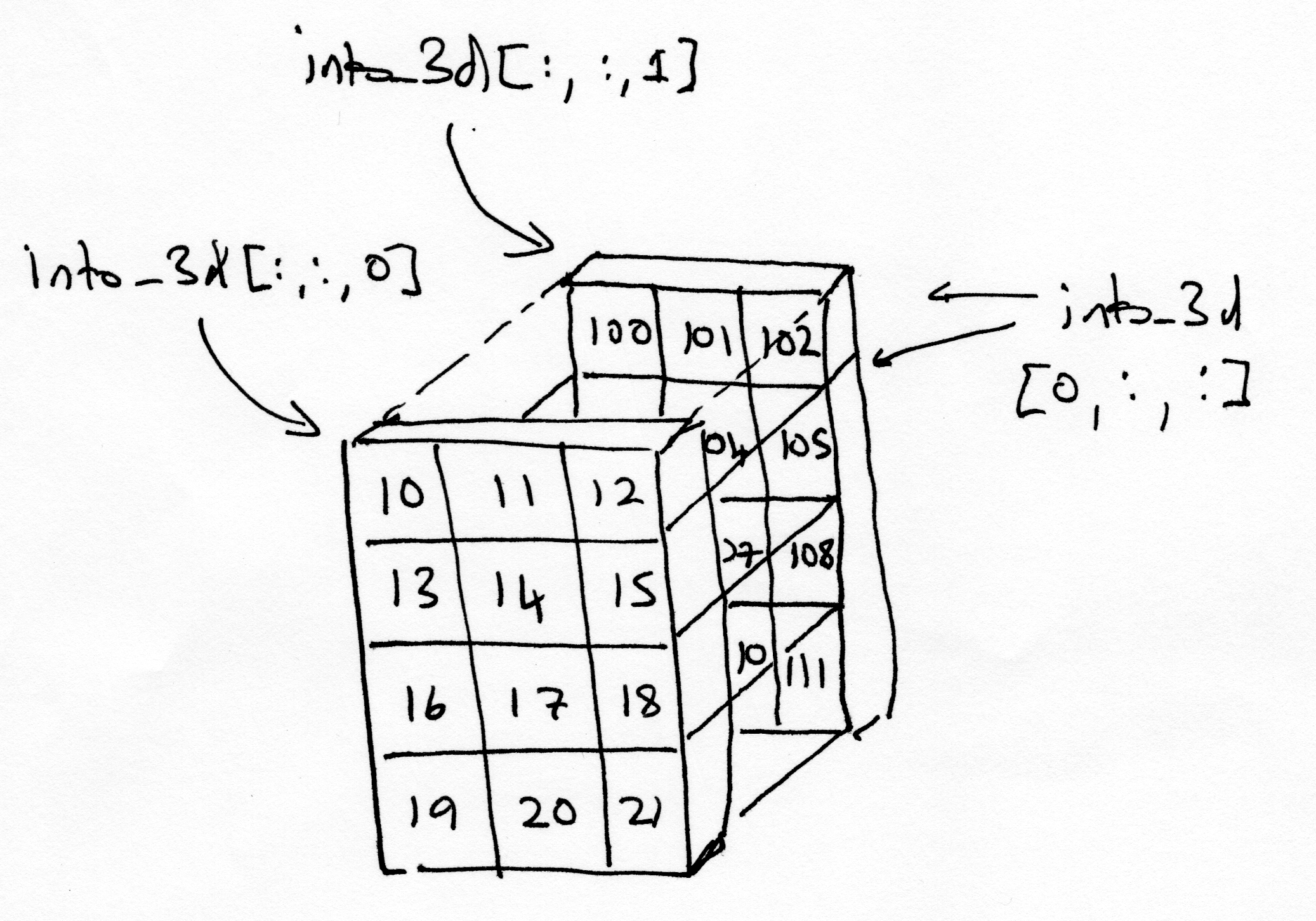
Relative to the images above, this is a different way of looking at the into_3d array, where the slices are in the first dimension, like this:

# First row, all columns, all planes.
into_3d[0, :, :]

array([[ 10, 100],
       [ 11, 101],
       [ 12, 102]])

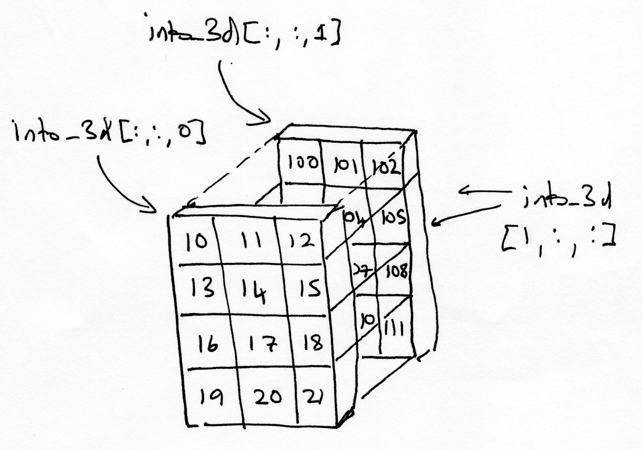
# Second row, all columns, all planes.
into_3d[1, :, :]

array([[ 13, 103],
       [ 14, 104],
       [ 15, 105]])

# Third row, all columns, all planes.
into_3d[2, :, :]

array([[ 16, 106],
       [ 17, 107],
       [ 18, 108]])

Make a prediction of what the values would look like by slicing in the second dimension.

Check your guess below:

# Your code here

Three-dimensional arrays

Contents

Three-dimensional arrays#

Two dimensions before three#

Three dimensions#